The Polymath15 paper “Effective approximation of heat flow evolution of the Riemann  function, and a new upper bound for the de Bruijn-Newman constant“, submitted to Research in the Mathematical Sciences, has just been uploaded to the arXiv. This paper records the mix of theoretical and computational work needed to improve the upper bound on the de Bruijn-Newman constant
  . This constant can be defined as follows. The function
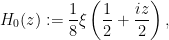
where is the Riemann function
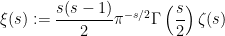
has a Fourier representation
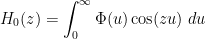
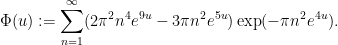
where  is the super-exponentially decaying function
The Riemann hypothesis is equivalent to the claim that all the zeroes of  are real. De Bruijn introduced (in different notation) the deformations

of ; one can view this as the solution to the backwards heat equation  starting at . From the work of de Bruijn and of Newman, it is known that there exists a real number – the de Bruijn-Newman constant – such that
  has all zeroes real for
  and has at least one non-real zero for
  . In particular, the Riemann hypothesis is equivalent to the assertion
  . Prior to this paper, the best known bounds for this constant were

with the lower bound due to Rodgers and myself, and the upper bound due to Ki, Kim, and Lee. One of the main results of the paper is to improve the upper bound to

At a purely numerical level this gets “closer” to proving the Riemann hypothesis, but the methods of proof take as input a finite numerical verification of the Riemann hypothesis up to some given height  (in our paper we take
  ) and converts this (and some other numerical verification) to an upper bound on that is of order
  . As discussed in the final section of the paper, further improvement of the numerical verification of RH would thus lead to modest improvements in the upper bound on , although it does not seem likely that our methods could for instance improve the bound to below
  without an infeasible amount of computation.
We now discuss the methods of proof. An existing result of de Bruijn shows that if all the zeroes of  lie in the strip
  , then
  ; we will verify this hypothesis with
  , thus giving (1). Using the symmetries and the known zero-free regions, it suffices to show that
whenever  and
and  .
.
For large  (specifically,
  ), we use effective numerical approximation to
  to establish (2), as discussed in a bit more detail below. For smaller values of , the existing numerical verification of the Riemann hypothesis (we use the results of Platt) shows that
for  and . The problem though is that this result only controls at time
  rather than the desired time
  . To bridge the gap we need to erect a “barrier” that, roughly speaking, verifies that
for  ,
,  , and ; with a little bit of work this barrier shows that zeroes cannot sneak in from the right of the barrier to the left in order to produce counterexamples to (2) for small .
To enforce this barrier, and to verify (2) for large , we need to approximate for positive  . Our starting point is the Riemann-Siegel formula, which roughly speaking is of the shape
where  ,
,  is an explicit “gamma factor” that decays exponentially in , and
  is a ratio of gamma functions that is roughly of size
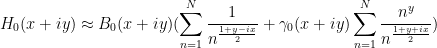
  . Deforming this by the heat flow gives rise to an approximation roughly of the form

where  and
and  are variants of and ,
  , and
, and  is an exponent which is roughly
 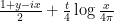 . In particular, for positive values of , increases (logarithmically) as increases, and the two sums in the Riemann-Siegel formula become increasingly convergent (even in the face of the slowly increasing coefficients
  ). For very large values of (in the range
  for a large absolute constant
  ), the
  terms of both sums dominate, and begins to behave in a sinusoidal fashion, with the zeroes “freezing” into an approximate arithmetic progression on the real line much like the zeroes of the sine or cosine functions (we give some asymptotic theorems that formalise this “freezing” effect). This lets one verify (2) for extremely large values of (e.g.,
  ). For slightly less large values of , we first multiply the Riemann-Siegel formula by an “Euler product mollifier” to reduce some of the oscillation in the sum and make the series converge better; we also use a technical variant of the triangle inequality to improve the bounds slightly. These are sufficient to establish (2) for moderately large (say ) with only a modest amount of computational effort (a few seconds after all the optimisations; on my own laptop with very crude code I was able to verify all the computations in a matter of minutes).
The most difficult computational task is the verification of the barrier (3), particularly when is close to zero where the series in (4) converge quite slowly. We first use an Euler product heuristic approximation to to decide where to place the barrier in order to make our numerical approximation to as large in magnitude as possible (so that we can afford to work with a sparser set of mesh points for the numerical verification). In order to efficiently evaluate the sums in (4) for many different values of  , we perform a Taylor expansion of the coefficients to factor the sums as combinations of other sums that do not actually depend on and
  and so can be re-used for multiple choices of after a one-time computation. At the scales we work in, this computation is still quite feasible (a handful of minutes after software and hardware optimisations); if one assumes larger numerical verifications of RH and lowers
  and
and  to optimise the value of accordingly, one could get down to an upper bound of
  assuming an enormous numerical verification of RH (up to height about
  ) and a very large distributed computing project to perform the other numerical verifications.
This post can serve as the (presumably final) thread for the Polymath15 project (continuing this post), to handle any remaining discussion topics for that project.


55 comments
Comments feed for this article
30 April, 2019 at 4:42 pm
ndwork
Congratulations to all!
30 April, 2019 at 7:09 pm
God's Geological/ Astrophysical Math Signs
neat stuff here ! I don’t understand it, but you got something going here!
1 May, 2019 at 4:10 am
Anonymous
The implied constant in the estimate

 )
)

(given that RH is verified up to height
seems to be close to
It would be interesting to find a good numerical upper bound on this constant (at least for sufficiently large ).
).
1 May, 2019 at 8:00 am
Terence Tao
Figure 20 in the writeup (and also Table 1) gives the numerical relationship between or
or  (which corresponds to
  ) and the upper bound for
  .
.
1 May, 2019 at 6:18 am
William Bauer
Congratulations from a camp follower.
1 May, 2019 at 8:44 am
MikeRuxton
Wikipedia de Bruijn-Newman constant page says
“In brief, the Riemann hypothesis is equivalent to the conjecture that Λ ≤ 0.”
Your intro says something different about Riemann hypothesis equivalence.
1 May, 2019 at 9:27 am
Anonymous
It can be equivalent to multiple things
1 May, 2019 at 3:26 pm
Joseph Sugar
So pushing down λ (e.g. below 0.1) is just another way of verifying that millions (depending on 0.1) of nontrivial zeros of the Zeta-function are on the critical line? Thanks.
1 May, 2019 at 4:21 pm
Anonymous
I think it’s the other way around, where verified zeros implies small lambda, not that small lambda implies verified zeros.
2 May, 2019 at 9:48 am
arch1
verified zeros plus the other two verifications (large x and barrier), right?
2 May, 2019 at 9:59 am
Anonymous
yes, verified zeros plus other stuff implies small lambda
1 May, 2019 at 7:28 pm
Lior Silberman
In the sentence about the work of de Bruijn and Newman you have the two cases as and
and  , but I think the second should be
[Corrected, thanks -T.]
2 May, 2019 at 7:02 am
Anonymous
In the extensive numerical study of zeros with
  , is there any evidence for the existence of a non-real multiple zero of
  for some
  ?
?
This question is motivated by the heuristic that it should be very unlikely (because of the strong "horizontal repelling" of nearby zeros) to have a non-real multiple zero of
  for any real
  .
.
2 May, 2019 at 9:38 am
Anonymous
Are the red and green tangencies double zeros in fig 19?
2 May, 2019 at 10:18 am
Anonymous
It seems that these tangencies represent only real zeros (since the y-coordinates at these tangencies are seen to be 0 – so these tangencies happen precisely when two “branches” representing the paths of two conjugate zeros are “colliding” on the real line.
A (hypothetical) non-real double zero in figure 19 should be similar but with its y-coordinate non-zero (obviously, there should be a corresponding conjugate non-real double zero with its y-coordinate having the same magnitude but different sign.)
3 May, 2019 at 4:19 pm
Terence Tao
As far as I know there is no numerical evidence of such a double zero, which should indeed be a very unlikely event (two complex equations in three real unknowns, with no functional equation to make one or more of the equations redundant).
6 May, 2019 at 4:22 am
Anonymous
Suppose that is non-real multiple zero of
  for some
  (which obviously requires
  ) such that
  for all
  .
. zeros) of the conjugate branches of
  for
for  near
near  , is it possible to show that there is always a branch of
  with its
  strictly increasing over a sufficiently small interval
  ?
?
By considering the Puiseux expansion (given by proposition 3.1(ii) on the dynamics of repeated
If true, it contradicts the assumption that for all
  – thereby showing that such
  must be a simple(!) zero of
  .
.
6 May, 2019 at 6:57 am
Terence Tao
Immediately after a repeated complex zero, the zeroes move in a mostly horizontal direction (becoming at distance about from their initial location for
  a little bit larger than
  ), but if the repeated zero was higher than all the other zeroes, they should also drift downwards. The latter effect gives a displacement of the order of
  , so the trajectories would then resemble a downward pointing parabola immediately after the double zero.
For a simple model to use as a specific numeric example, one can try the initial polynomial that has a repeated zero at
  . The backwards heat flow for this is
which has zeroes at (if I did not make any numerical errors) and one should be able to plot these trajectories explicitly.
2 May, 2019 at 8:59 am
arch1
“…counterexamples to (2) to small x” ->
“…counterexamples to (2) for small x”
[Corrected, thanks – T.]
3 May, 2019 at 1:51 am
Vincent
A naive question from a non-native speaker. When you write
“From the work of de Bruijn and of Newman, it is known that there exists a real number {\Lambda} – the de Bruijn-Newman constant – such that {H_t} has purely real zeroes for {t \geq \Lambda} …”
does this mean that {H_t} has NO purely real zeroes for {t} strictly less than {\Lambda} or just that based on the work of de Bruijn and Newman we can’t (or won’t) say anything about zeroes for t smaller than {\Lambda}?
Given the equivalence to the Riemann hypothesis further down the text I think the first of the two possibilities is intended, but as I read the sentence by itself the latter interpretation seems more plausible. If indeed the former interpretation is correct, then where lies my mistake, i.e. what is the general linguistic rule at work here?
3 May, 2019 at 2:02 am
Vincent
I just read the abstract on Arxiv and now I think the source of my confusion lies somewhere else than I thought. The text of the blog suggests that for t as least as big Lambda we have some purely real zeroes, but, except possibly in the case of t exactly equal to Lambda, they are accompanied by some non-real zeroes as well. Now Arxiv says that this latter statement is false, and that probably you meant to write that the non-real zeroes appear for t SMALLER than lambda. Is that correct? I guess this is also the content of Lior Silberman’s comment above that somehow refuses to parse in my browser.
[Text reworded – T.]
3 May, 2019 at 4:37 am
Anonymous
In the arxiv paper, in the line below (2), it seems clearer to replace “after removing all the singularities” by “after removing all trivial zeros and the singularity at “.
“.
[Thanks, this will be reworded in the next revision of the ms -T.]
3 May, 2019 at 5:07 am
Anonymous
In the arxiv paper, in remark 8.3, it seems clearer to add a definition of the “imaginary error function” erfi.
[Thanks, this will be done in the next revision of the ms -T.]
3 May, 2019 at 9:02 am
Anonymous
I know this is out of context but I don’t know the best place to ask the following: can you infer something more important from what is on the link below?
– Are prime numbers really random?
https://math.stackexchange.com/q/3113307
3 May, 2019 at 10:50 am
rudolph01
The connection between the height of the RH verification and the achieved, actually is the result of the approach we chose. However, to achieve a lower
  we don’t have to verify the RH at
  , but only that the ‘elevated’
  -rectangle
  at
at  is zero free (with
  is the Barrier location). The work of Platt, Gourdon et al made this a very convenient choice, that only came at a small ‘cost’ of needing to introduce a Barrier to prevent zeros flying ‘under the elevated roof’ from the right.
I wondered whether the recently developed approach to verify the right side of the Barrier ‘roof’, could also be applied to (part of) its left side, thereby making the Barrier itself obsolete? Or will we run into trouble with the bound and/or the error terms at lower ? (I do recall the error terms became too large around
  ).
).
5 May, 2019 at 7:35 am
rudolph01
Ah wait, that won’t work since the Lemma-bound will become negative at some point left of the Barrier and we can’t just add mollifiers to make it positive again ( at 6 primes was the lowest positive bound I managed to achieve).
Even though it appears to be a bit of an ‘overkill’, verifying the RH using its already optimised techniques (Gram/Rosser’s law, Turing’s method, etc), is probably always going to beat some form of applying the argument principle to the ‘elevated’, smaller rectangle at …
…
6 May, 2019 at 7:01 am
Terence Tao
Also, numerical verification of RH has many orders of magnitude more applications than verification of zero free-region of at some distance
  away from the critical line, so if one were to undertake a massive computational effort, it would be much more useful to direct it towards the former rather than the latter. :)
9 May, 2019 at 4:08 am
Anonymous
In the arxiv paper, it seems that in (28) (and also in its proof)
 should be an ordinary derivative
Similar corrections are needed for (34) (the function ) and perhaps remark 9.4
[Corrected, thanks – T.]
12 May, 2019 at 1:07 pm
Anonymous
Is this polymath over?
17 June, 2019 at 6:19 am
Anonymous
It is interesting to observe that the dynamics of zeros is quite similar to the “guiding equation” dynamics of particles in De Broglie – Bohm theory (for a deterministic non-local interpretation of quantum mechanics), see
https://en.wikipedia.org/wiki/De_Broglie-Bohm_theory
In which the 3D deterministic guiding equation for the particles (based on a wave function satisfying Schrodinger equation which is similar to the heat equation satisfied by
  ) is similar to
  zero dynamics. It seems that
  plays the role of a “wave function” which determine the dynamics of its own zeros (interpreted as particles).
 zeros.
As is well-known, the predictions of De Broglie – Bohm theory are completely consistent with the standard interpretation of quantum mechanics, it seems that this analogy may explain certain “probabilistic properties” of the dynamics of
18 June, 2019 at 12:08 am
Anonymous
It seems that the approximations of in the critical strip by elementary functions is perhaps less efficient than similar approximations of the slightly modified function
  for sufficiently large
  because the distribution of its zeros is more uniform (the number of its zeros up to
  grows asymptotically linearly with
  while growing like
  for
for  ) – so it seems more adapted for asymptotic approximations by elementary functions.
25 July, 2019 at 3:47 pm
Terence Tao
Update from the submission: we received two positive referee reports on the paper with some minor corrections suggested at https://terrytao.files.wordpress.com/2019/07/de-bruijn-newman-report.pdf and https://terrytao.files.wordpress.com/2019/07/condensed-review.pdf . I should be able to attend to these changes and send back the revision soon.
26 July, 2019 at 8:09 am
Anonymous
congratulations! and that second reviewer’s attention to detail
26 July, 2019 at 1:29 pm
Terence Tao
Yes, that referee certainly went through many of the calculations in fine detail! I have implemented the corrections and am now returning it back to the journal.
26 July, 2019 at 2:19 pm
Anonymous
Congratulations on your papers’ submissions!
And are you now convinced that the Riemann Hypothesis is true?
27 July, 2019 at 6:51 am
Anonymous
The constant moved from 0.50 to 0.22 and when it reaches 0.00 the Riemann hypothesis is proved, so we have progressed 56% of the way to proving the Riemann hypothesis. Analytic number theorists call that amusing. Other academics call that a mnemonic. Bureaucrats call that a metric.
28 July, 2019 at 5:18 am
rudolph01
After Rodgers and Tao showed last year that , we know that Newman’s conjecture that “if the RH is true, then it is barely so” has become true. However, even with a reduced upper bound of
  there is still plenty of room for the conjecture: “if the RH is false, then it could be considerably so”… ;-)
1 August, 2019 at 9:43 am
Terence Tao
The paper has now been accepted for publication in RIMS.
4 August, 2019 at 1:33 am
Anonymous
The arXiv paper is still not updated.
[Thanks for the reminder! I have sent in an update and it should appear in a day or two. -T]
6 August, 2019 at 1:44 pm
Anonymous
Some typos in the updated arXiv paper: ,
,  should be
  and for
  , “
, “ ” should be corrected.
 should be
  .
.
In page 13, for
In page 66, in the explanation of figure 20,
[Thanks, this will be corrected in the next revision of the ms. -T]
27 July, 2019 at 6:18 am
Anonymous
Dear Terry
I have a girlfriend and I always talk to her that until Pro. Tao receives $1M from Clay Millenium award , I take her to 10 nations in the world
27 July, 2019 at 7:11 am
Raphael
I find this solid/liquid/gaseous analogy highly inspiring. It brings me to the following question: What is the structure of a crystalline solid substance exactly at the melting point? In the solid it will be anything with a discrete diffraction pattern (say Fourier transform) and highly anisotropic (in general at least for n>1 dimensions) in the liquid it will be isotroic (radially symmetric diffraction pattern) and be determined by statistical properties like average distances and higher momenta of the distribution. I suspect regarding exactly the melting point will be severely hampered by discontinuities of characterizing properties. For example free energy or other thermodynamic properties have cusps at the melting point. Maybe one has to uncover what is hidden behind such “discontinuities” to understand what is going on at the phase border. Possibly the structure at the melting point is something analogous to the distribution of the zeros of the -function?
25 August, 2019 at 9:08 pm
Anonymous
The Riemann Hypothesis is true!
26 August, 2019 at 11:20 am
Anonymous
Yes! The Riemann Hypothesis is true!
The Goldbach conjecture is also true!
The ABC conjecture is also true!
The Collatz conjecture is also true!
The Polignac conjecture is also true!
…
Why? I proved those conjecture are true!
David Cole
https://www.researchgate.net/profile/David_Cole29
https://www.math10.com/forum/viewforum.php?f=63&sid=0f36c9b09298e37868fc5eb2adea1a06
26 August, 2019 at 11:22 am
Anonymous
Fermat’s Last Theorem is also true too!
https://math.stackexchange.com/questions/1993460/prove-a-statement-about-a-conditional-diophantine-equation
David Cole.
26 August, 2019 at 2:36 pm
Anonymous
Life is not fair!…. :-(
10 September, 2019 at 2:46 pm
rudolph01
I wondered whether other functions than exist that also involve
  and possess similar properties. in particular being real-valued when
  and having a Fourier representation that could be perturbed by the time-factor
  .
.
A potentially interesting one is:
that induces an extra set of more regularly spaced zeros on top of the non-trivial zeros
  . Also, by adding an additional parameter
  as follows:
it seems possible to increase the density of these ‘s whilst keeping them on the critical line.
Just for fun, I dusted off some of the software tools used in our Polymath 15 project to see whether there was something interesting about the trajectories of these zeros over ‘time’. To keep this post short, I have summarised my observations in a few visuals in the link:
PPT
PDF
Open to feedback/suggestions.
27 September, 2019 at 10:19 am
rudolph01
Did some further computations. Suppose the regularly spaced are indeed all real at
  , then when their density is increased through parameter
  :
:
1) collisions at negative appear to occur closer to
  . This could be explained by the fact that when the density of the
  ‘s increases, they will get closer to the (fixed)
  ‘s and form “Lehmer-like”-pairs at
  . This phenomenon would imply the lower bound of
  moves up when
  increases.
2) collisions at positive are difficult to test since we don’t have a
  lying off the critical line. However, after injecting a ‘fake’
  close to the edge of the strip, the data shows that its associated collision will occur ‘sooner’. This could be explained by the trajectories of the real zeros eventually all leaning in the north-western direction. So, when more
  -trajectories are induced, more of these trajectories will travel above than below the collision point associated to
  . Hence that point experiences a downward pressure towards
  and this would imply the upper bound of
  moves down when
  increases.
The observations above do not yield any new insights about where the
  ‘s and the
  ’s are just ‘givens’ that are perturbed into the positive and negative
  -directions (i.e. all information originates from
  and nothing flows back).
Updated pdf.
Asked about the ‘s
‘s
at mathoverflow.
27 September, 2019 at 11:31 am
Anonymous
It seems that by using asymptotic approximations (with remainder term) for the function whose zeros are the ‘s, it is possible to get asymptotic approximation for the
  – trajectories. The derivation of the aymptotic approximation of this function may use the known asymptotic form (with remainder term) of the
  function (as done in Polymath15 paper.)
22 April, 2020 at 12:36 pm
Terence Tao
Just a small comment to note that there has been a recent numerical verification of RH up to height in https://arxiv.org/abs/2004.09765 which, among other things, immediately improves the upper bound
  in the Polymath15 paper to
  .
.
22 April, 2020 at 10:26 pm
Anonymous
“Just a small comment” :)
22 April, 2020 at 11:40 pm
goingtoinfinity
Are there any ways to confirm the verification of RH up to the said point? More precisely, does the calculation produce data points that can be used for verification of the result in significantly less time than it would take to run the verification again? (simplest example would be prime factorization, which can easily be checked afterwards).
23 April, 2020 at 7:34 am
Terence Tao
This is a good question. I think with our current technology any verification of RH up to height is going to need something like
  steps, so it’s not going to be quickly replicable. In principle one could maybe convert their verification into some enormous probabilistically checkable proof or something, but that seems more effort than it is really worth. On the other hand having some “checksums” (e.g. collecting some statistics of the zeroes computed) might be doable without having to run the entire code again. But one would have to contact the authors about this; I didn’t see much discussion of these topics in the paper itself.
1 May, 2020 at 10:39 am
Rudolph
From the paper: “(…)The next entry in Table 1 of [24] is conditional on taking a little higher than
  , which of course, is not achieved by Theorem 1. This would enable one to prove
  . Given that our value of
  falls between the entries in this table, it is possible that some extra decimals could be wrought out of the calculation. We have not pursued this(…)”
This is not so difficult to pursue. The new RH-verification height translates into
  (since
  ) and
) and  . At this
  , the mollified triangle lower bound becomes and stays larger than
  for the choice
  . These yield a
  , and to be on the safe side let’s take
  (note that slightly different choices for
  might lead to a further reduction).
With these parameters, an optimal barrier location can be established, i.e. where shows a larger peak. It turns out that
  is a suitable location. Then running the barrier computations yields a winding number of
  , so that we have verified that no complex zeros could have flown through the barrier from the right and no zeros could have flown in through the bottom at
  on its left, since the RH has been verified up that point.
Barrier computation output
29 July, 2021 at 10:31 pm
Raphael
Gaseous implies the existence of a complex conjugate pair of zeros of $ latex H_t $, while liquid implies purely real zeros. What would the phase border gaseous/liquid look like? Would it imply the existence of zeros of order >1 (say 2)? If so, and if there is an operator whose eigenvalues are the zeros, what symmetry properties (which symmetry goup) would this operator have (belong to)? I suppose it would be a just about non-, abelian group. Because the eigenvalue “degeneracy” reflects the non-abelianess of the corresponding symmetry group. Do such operators exist, or can we construct such operators?