What are the odds?

3 October, 2022 in diversions, expository, math.PR, math.ST | Tags: Bayesian probability, lotteries | by Terence Tao

An unusual lottery result made the news recently: on October 1, 2022, the PCSO Grand Lotto in the Philippines, which draws six numbers from ${1}$ to ${55}$ at random, managed to draw the numbers ${9, 18, 27, 36, 45, 54}$ (though the balls were actually drawn in the order ${9, 45,36, 27, 18, 54}$ ). In other words, they drew exactly six multiples of nine from ${1}$ to ${55}$ . In addition, a total of ${433}$ tickets were bought with this winning combination, whose owners then had to split the ${236}$ million peso jackpot (about ${4}$ million USD) among themselves. This raised enough suspicion that there were calls for an inquiry into the Philippine lottery system, including from the minority leader of the Senate.

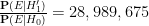
Whenever an event like this happens, journalists often contact mathematicians to ask the question: “What are the odds of this happening?”, and in fact I myself received one such inquiry this time around. This is a number that is not too difficult to compute – in this case, the probability of the lottery producing the six numbers ${9, 18, 27, 35, 45, 54}$ in some order turn out to be ${1}$ in ${\binom{55}{6} = 28,989,675}$ – and such a number is often dutifully provided to such journalists, who in turn report it as some sort of quantitative demonstration of how remarkable the event was.

But on the previous draw of the same lottery, on September 28, 2022, the unremarkable sequence of numbers ${11, 26, 33, 45, 51, 55}$ were drawn (again in a different order), and no tickets ended up claiming the jackpot. The probability of the lottery producing the six numbers ${11, 26, 33, 45, 51, 55}$ is also ${1}$ in ${\binom{55}{6} = 28,989,675}$ – just as likely or as unlikely as the October 1 numbers ${9, 18, 27, 36, 45, 54}$ . Indeed, the whole point of drawing the numbers randomly is to make each of the ${28,989,675}$ possible outcomes (whether they be “unusual” or “unremarkable”) equally likely. So why is it that the October 1 lottery attracted so much attention, but the September 28 lottery did not?

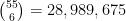
Part of the explanation surely lies in the unusually large number ( ${433}$ ) of lottery winners on October 1, but I will set that aspect of the story aside until the end of this post. The more general points that I want to make with these sorts of situations are:

The question “what are the odds of happening” is often easy to answer mathematically, but it is not the correct question to ask.
The question “what is the probability that an alternative hypothesis is the truth” is (one of) the correct questions to ask, but is very difficult to answer (it involves both mathematical and non-mathematical considerations).
The answer to the first question is one of the quantities needed to calculate the answer to the second, but it is far from the only such quantity. Most of the other quantities involved cannot be calculated exactly.
However, by making some educated guesses, one can still sometimes get a very rough gauge of which events are “more surprising” than others, in that they would lead to relatively higher answers to the second question.

To explain these points it is convenient to adopt the framework of Bayesian probability. In this framework, one imagines that there are competing hypotheses to explain the world, and that one assigns a probability to each such hypothesis representing one’s belief in the truth of that hypothesis. For simplicity, let us assume that there are just two competing hypotheses to be entertained: the null hypothesis ${H_0}$ , and an alternative hypothesis ${H_1}$ . For instance, in our lottery example, the two hypotheses might be:

Null hypothesis ${H_0}$ : The lottery is run in a completely fair and random fashion.
Alternative hypothesis ${H_1}$ : The lottery is rigged by some corrupt officials for their personal gain.

At any given point in time, a person would have a probability ${{\bf P}(H_0)}$ assigned to the null hypothesis, and a probability ${{\bf P}(H_1)}$ assigned to the alternative hypothesis; in this simplified model where there are only two hypotheses under consideration, these probabilities must add to one, but of course if there were additional hypotheses beyond these two then this would no longer be the case.

Bayesian probability does not provide a rule for calculating the initial (or prior) probabilities ${{\bf P}(H_0)}$ , ${{\bf P}(H_1)}$ that one starts with; these may depend on the subjective experiences and biases of the person considering the hypothesis. For instance, one person might have quite a bit of prior faith in the lottery system, and assign the probabilities ${{\bf P}(H_0) = 0.99}$ and ${{\bf P}(H_1) = 0.01}$ . Another person might have quite a bit of prior cynicism, and perhaps assign ${{\bf P}(H_0)=0.5}$ and ${{\bf P}(H_1)=0.5}$ . One cannot use purely mathematical arguments to determine which of these two people is “correct” (or whether they are both “wrong”); it depends on subjective factors.

What Bayesian probability does do, however, is provide a rule to update these probabilities ${{\bf P}(H_0)}$ , ${{\bf P}(H_1)}$ in view of new information ${E}$ to provide posterior probabilities ${{\bf P}(H_0|E)}$ , ${{\bf P}(H_1|E)}$ . In our example, the new information ${E}$ would be the fact that the October 1 lottery numbers were ${9, 18, 27, 36, 45, 54}$ (in some order). The update is given by the famous Bayes theorem

$\displaystyle {\bf P}(H_0|E) = \frac{{\bf P}(E|H_0) {\bf P}(H_0)}{{\bf P}(E)}; \quad {\bf P}(H_1|E) = \frac{{\bf P}(E|H_1) {\bf P}(H_1)}{{\bf P}(E)},$

where ${{\bf P}(E|H_0)}$ is the probability that the event ${E}$ would have occurred under the null hypothesis ${H_0}$ , and ${{\bf P}(E|H_1)}$ is the probability that the event ${E}$ would have occurred under the alternative hypothesis ${H_1}$ . Let us divide the second equation by the first to cancel the ${{\bf P}(E)}$ denominator, and obtain

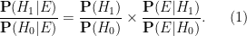
$\displaystyle \frac{ {\bf P}(H_1|E) }{ {\bf P}(H_0|E) } = \frac{ {\bf P}(H_1) }{ {\bf P}(H_0) } \times \frac{ {\bf P}(E | H_1)}{{\bf P}(E | H_0)}. \ \ \ \ \ (1)$

One can interpret ${\frac{ {\bf P}(H_1) }{ {\bf P}(H_0) }}$ as the prior odds of the alternative hypothesis, and ${\frac{ {\bf P}(H_1|E) }{ {\bf P}(H_0|E) } }$ as the posterior odds of the alternative hypothesis. The identity (1) then says that in order to compute the posterior odds ${\frac{ {\bf P}(H_1|E) }{ {\bf P}(H_0|E) }}$ of the alternative hypothesis in light of the new information ${E}$ , one needs to know three things:

The prior odds ${\frac{ {\bf P}(H_1) }{ {\bf P}(H_0) }}$ of the alternative hypothesis;
The probability ${\mathop{\bf P}(E|H_0)}$ that the event ${E}$ occurs under the null hypothesis ${H_0}$ ; and
The probability ${\mathop{\bf P}(E|H_1)}$ that the event ${E}$ occurs under the alternative hypothesis ${H_1}$ .

As previously discussed, the prior odds ${\frac{ {\bf P}(H_1) }{ {\bf P}(H_0) }}$ of the alternative hypothesis are subjective and vary from person to person; in the example earlier, the person with substantial faith in the lottery may only give prior odds of ${\frac{0.01}{0.99} \approx 0.01}$ (99 to 1 against) of the alternative hypothesis, whereas the cynic might give odds of ${\frac{0.5}{0.5}=1}$ (even odds). The probability ${{\bf P}(E|H_0)}$ is the quantity that can often be calculated by straightforward mathematics; as discussed before, in this specific example we have

$\displaystyle \mathop{\bf P}(E|H_0) = \frac{1}{\binom{55}{6}} = \frac{1}{28,989,675}.$

But this still leaves one crucial quantity that is unknown: the probability ${{\bf P}(E|H_1)}$ . This is incredibly difficult to compute, because it requires a precise theory for how events would play out under the alternative hypothesis ${H_1}$ , and in particular is very sensitive as to what the alternative hypothesis ${H_1}$ actually is.

For instance, suppose we replace the alternative hypothesis ${H_1}$ by the following very specific (and somewhat bizarre) hypothesis:

Alternative hypothesis ${H'_1}$ : The lottery is rigged by a cult that worships the multiples of ${9}$ , and views October 1 as their holiest day. On this day, they will manipulate the lottery to only select those balls that are multiples of ${9}$ .

Under this alternative hypothesis ${H'_1}$ , we have ${{\bf P}(E|H'_1)=1}$ . So, when ${E}$ happens, the odds of this alternative hypothesis ${H'_1}$ will increase by the dramatic factor of ${\frac{{\bf P}(E|H'_1)}{{\bf P}(E|H_0)} = 28,989,675}$ . So, for instance, someone who already was entertaining odds of ${\frac{0.01}{0.99}}$ of this hypothesis ${H'_1}$ would now have these odds multiply dramatically to ${\frac{0.01}{0.99} \times 28,989,675 \approx 290,000}$ , so that the probability of ${H'_1}$ would have jumped from a mere ${1\%}$ to a staggering ${99.9997\%}$ . This is about as strong a shift in belief as one could imagine. However, this hypothesis ${H'_1}$ is so specific and bizarre that one’s prior odds of this hypothesis would be nowhere near as large as ${\frac{0.01}{0.99}}$ (unless substantial prior evidence of this cult and its hold on the lottery system existed, of course). A more realistic prior odds for ${H'_1}$ would be something like ${\frac{10^{-10^{10}}}{1-10^{-10^{10}}}}$ – which is so miniscule that even multiplying it by a factor such as ${28,989,675}$ barely moves the needle.

Remark 1 The contrast between alternative hypothesis ${H_1}$ and alternative hypothesis ${H'_1}$ illustrates a common demagogical rhetorical technique when an advocate is trying to convince an audience of an alternative hypothesis, namely to use suggestive language (“`I’m just asking questions here”) rather than precise statements in order to leave the alternative hypothesis deliberately vague. In particular, the advocate may take advantage of the freedom to use a broad formulation of the hypothesis (such as ${H_1}$ ) in order to maximize the audience’s prior odds of the hypothesis, simultaneously with a very specific formulation of the hypothesis (such as ${H'_1}$ ) in order to maximize the probability of the actual event ${E}$ occuring under this hypothesis. (A related technique is to be deliberately vague about the hypothesized competency of some suspicious actor, so that this actor could be portrayed as being extraordinarily competent when convenient to do so, while simultaneously being portrayed as extraordinarily incompetent when that instead is the more useful hypothesis.) This can lead to wildly inaccurate Bayesian updates of this vague alternative hypothesis, and so precise formulation of such hypothesis is important if one is to approach a topic from anything remotely resembling a scientific approach. [EDIT: as pointed out to me by a reader, this technique is a Bayesian analogue of the motte and bailey fallacy.]

At the opposite extreme, consider instead the following hypothesis:

Alternative hypothesis ${H''_1}$ : The lottery is rigged by some corrupt officials, who on October 1 decide to randomly determine the winning numbers in advance, share these numbers with their collaborators, and then manipulate the lottery to choose those numbers that they selected.

If these corrupt officials are indeed choosing their predetermined winning numbers randomly, then the probability ${{\bf P}(E|H''_1)}$ would in fact be just the same probability ${\frac{1}{\binom{55}{6}} = \frac{1}{28,989,675}}$ as ${{\bf P}(E|H_0)}$ , and in this case the seemingly unusual event ${E}$ would in fact have no effect on the odds of the alternative hypothesis, because it was just as unlikely for the alternative hypothesis to generate this multiples-of-nine pattern as for the null hypothesis to. In fact, one would imagine that these corrupt officials would avoid “suspicious” numbers, such as the multiples of ${9}$ , and only choose numbers that look random, in which case ${{\bf P}(E|H''_1)}$ would in fact be less than ${{\bf P}(E|H_0)}$ and so the event ${E}$ would actually lower the odds of the alternative hypothesis in this case. (In fact, one can sometimes use this tendency of fraudsters to not generate truly random data as a statistical tool to detect such fraud; violations of Benford’s law for instance can be used in this fashion, though only in situations where the null hypothesis is expected to obey Benford’s law, as discussed in this previous blog post.)

Now let us consider a third alternative hypothesis:

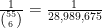
Alternative hypothesis ${H'''_1}$ : On October 1, the lottery machine developed a fault and now only selects numbers that exhibit unusual patterns.

Setting aside the question of precisely what faulty mechanism could induce this sort of effect, it is not clear at all how to compute ${{\bf P}(E|H'''_1)}$ in this case. Using the principle of indifference as a crude rule of thumb, one might expect

$\displaystyle {\bf P}(E|H'''_1) \approx \frac{1}{\# \{ \hbox{unusual patterns}\}}$

where the denominator is the number of patterns among the possible ${\binom{55}{6}}$ lottery outcomes that are “unusual”. Among such patterns would presumably be the multiples-of-9 pattern ${9,18,27,36,45,54}$ , but one could easily come up with other patterns that are equally “unusual”, such as consecutive strings such as ${11, 12, 13, 14, 15, 16}$ , or the first few primes ${2, 3, 5, 7, 11, 13}$ , or the first few squares 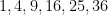${1, 4, 9, 16, 25, 36}$ , and so forth. How many such unusual patterns are there? This is too vague a question to answer with any degree of precision, but as one illustrative statistic, the Online Encyclopedia of Integer Sequences (OEIS) currently hosts about ${350,000}$ sequences. Not all of these would begin with six distinct numbers from ${1}$ to ${55}$ , and several of these sequences might generate the same set of six numbers, but this does suggests that patterns that one would deem to be “unusual” could number in the thousands, tens of thousands, or more. Using this guess, we would then expect the event ${E}$ to boost the odds of this hypothesis ${H'''_1}$ by perhaps a thousandfold or so, which is moderately impressive. But subsequent information can counteract this effect. 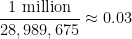For instance, on October 3, the same lottery produced the numbers ${8, 10, 12, 14, 26, 51}$ , which exhibit no unusual properties (no search results in the OEIS, for instance); if we denote this event by ${E'}$ , then we have ${{\bf P}(E'|H'''_1) \approx 0}$ and so this new information ${E'}$ should drive the odds for this alternative hypothesis ${H'''_1}$ way down again.

Remark 2 This example demonstrates another demagogical rhetorical technique that one sometimes sees (particularly in political or other emotionally charged contexts), which is to cherry-pick the information presented to their audience by informing them of events ${E}$ which have a relatively high probability of occurring under their alternative hypothesis, but withholding information about other relevant events ${E'}$ that have a relatively low probability of occurring under their alternative hypothesis. When confronted with such new information ${E'}$ , a common defense of a demogogue is to modify the alternative hypothesis ${H_1}$ to a more specific hypothesis ${H'_1}$ that can “explain” this information ${E'}$ (“Oh, clearly we heard about ${E'}$ because the conspiracy in fact extends to the additional organizations ${X, Y, Z}$ that reported ${E'}$ “), taking advantage of the vagueness discussed in Remark 1.

Let us consider a superficially similar hypothesis:

Alternative hypothesis ${H''''_1}$ : On October 1, a divine being decided to send a sign to humanity by placing an unusual pattern in a lottery.

Here we (literally) stay agnostic on the prior odds of this hypothesis, and do not address the theological question of why a divine being should choose to use the medium of a lottery to send their signs. At first glance, the probability ${{\bf P}(E|H''''_1)}$ here should be similar to the probability ${{\bf P}(E|H'''_1)}$ , and so perhaps one could use this event ${E}$ to improve the odds of the existence of a divine being by a factor of a thousand or so. But note carefully that the hypothesis ${H''''_1}$ did not specify which lottery the divine being chose to use. The PSCO Grand Lotto is just one of a dozen lotteries run by the Philippine Charity Sweepstakes Office (PCSO), and of course there are over a hundred other countries and thousands of states within these countries, each of which often run their own lotteries. Taking into account these thousands or tens of thousands of additional lotteries to choose from, the probability ${{\bf P}(E|H''''_1)}$ now drops by several orders of magnitude, and is now basically comparable to the probability ${{\bf P}(E|H_0)}$ coming from the null hypothesis. As such one does not expect the event ${E}$ to have a significant impact on the odds of the hypothesis ${H''''_1}$ , despite the small-looking nature ${\frac{1}{28,989,675}}$ of the probability ${{\bf P}(E|H_0)}$ .

In summary, we have failed to locate any alternative hypothesis ${H_1}$ which

Has some non-negligible prior odds of being true (and in particular is not excessively specific, as with hypothesis ${H'_1}$ );
Has a significantly higher probability of producing the specific event ${E}$ than the null hypothesis; AND
Does not struggle to also produce other events ${E'}$ that have since been observed.

One needs all three of these factors to be present in order to significantly weaken the plausibility of the null hypothesis ${H_0}$ ; in the absence of these three factors, a moderately small numerical value of ${{\bf P}(E|H_0)}$ , such as ${\frac{1}{28,989,675}}$ does not actually do much to affect this plausibility. In this case one needs to lay out a reasonably precise alternative hypothesis ${H_1}$ and make some actual educated guesses towards the competing probability ${{\bf P}(E|H_1)}$ before one can lead to further conclusions. However, if ${{\bf P}(E|H_0)}$ is insanely small, e.g., less than ${10^{-1000}}$ , then the possibility of a previously overlooked alternative hypothesis ${H_1}$ becomes far more plausible; as per the famous quote of Arthur Conan Doyle’s Sherlock Holmes, “When you have eliminated all which is impossible, then whatever remains, however improbable, must be the truth.”

We now return to the fact that for this specific October 1 lottery, there were ${433}$ tickets that managed to select the winning numbers. Let us call this event ${F}$ . In view of this additional information, we should now consider the ratio of the probabilities ${{\bf P}(E \& F|H_1)}$ and ${{\bf P}(E \& F|H_0)}$ , rather than the ratio of the probabilities ${{\bf P}(E|H_1)}$ and ${{\bf P}(E|H_0)}$ . If we augment the null hypothesis to

Null hypothesis ${H'_0}$ : The lottery is run in a completely fair and random fashion, and the purchasers of lottery tickets also select their numbers in a completely random fashion.

Then ${{\bf P}(E \& F|H'_0)}$ is indeed of the “insanely improbable” category mentioned previously. I was not able to get official numbers on how many tickets are purchased per lottery, but let us say for sake of argument that it is 1 million (the conclusion will not be extremely sensitive to this choice). Then the expected number of tickets that would have the winning numbers would be

$\displaystyle \frac{1 \hbox{ million}}{28,989,675} \approx 0.03$

(which is broadly consistent, by the way, with the jackpot being reached every ${30}$ draws or so), and standard probability theory suggests that the number of winners should now follow a Poisson distribution with this mean ${\lambda = 0.03}$ . The probability of obtaining ${433}$ winners would now be

$\displaystyle {\bf P}(F|H'_0) = \frac{\lambda^{433} e^{-\lambda}}{433!} \approx 10^{-1600}$

and of course ${{\bf P}(E \& F|H'_0)}$ would be even smaller than this. So this clearly demands some sort of explanation. But in actuality, many purchasers of lottery tickets do not select their numbers completely randomly; they often have some “lucky” numbers (e.g., based on birthdays or other personally significant dates) that they prefer to use, or choose numbers according to a simple pattern rather than go to the trouble of trying to make them truly random. So if we modify the null hypothesis to

Null hypothesis ${H''_0}$ : The lottery is run in a completely fair and random fashion, but a significant fraction of the purchasers of lottery tickets only select “unusual” numbers.

then it can now become quite plausible that a highly unusual set of numbers such as ${9,18,27,36,45,54}$ could be selected by as many as ${433}$ purchasers of tickets; for instance, if ${10\%}$ of the 1 million ticket holders chose to select their numbers according to some sort of pattern, then only ${0.4\%}$ of those holders would have to pick ${9,18,27,36,45,54}$ in order for the event ${F}$ to hold (given ${E}$ ), and this is not extremely implausible. Given that this reasonable version of the null hypothesis already gives a plausible explanation for ${F}$ , there does not seem to be a pressing need to locate an alternate hypothesis ${H_1}$ that gives some other explanation (cf. Occam’s razor). [UPDATE: Indeed, given the actual layout of the tickets of ths lottery, the numbers ${9,18,27,35,45,54}$ form a diagonal, and so all that is needed in order for the modified null hypothesis ${H''_0}$ to explain the event ${F}$ is to postulate that a significant fraction of ticket purchasers decided to lay out their numbers in a simple geometric pattern, such as a row or diagonal.]

Remark 3 In view of the above discussion, one can propose a systematic way to evaluate (in as objective a fashion as possible) rhetorical claims in which an advocate is presenting evidence to support some alternative hypothesis:

State the null hypothesis ${H_0}$ and the alternative hypothesis ${H_1}$ as precisely as possible. In particular, avoid conflating an extremely broad hypothesis (such as the hypothesis ${H_1}$ in our running example) with an extremely specific one (such as ${H'_1}$ in our example).
With the hypotheses precisely stated, give an honest estimate to the prior odds of this formulation of the alternative hypothesis.
Consider if all the relevant information ${E}$ (or at least a representative sample thereof) has been presented to you before proceeding further. If not, consider gathering more information ${E'}$ from further sources.
Estimate how likely the information ${E}$ was to have occurred under the null hypothesis.
Estimate how likely the information ${E}$ was to have occurred under the alternative hypothesis (using exactly the same wording of this hypothesis as you did in previous steps).
If the second estimate is significantly larger than the first, then you have cause to update your prior odds of this hypothesis (though if those prior odds were already vanishingly unlikely, this may not move the needle significantly). If not, the argument is unconvincing and no significant adjustment to the odds (except perhaps in a downwards direction) needs to be made.

55 comments

Comments feed for this article

3 October, 2022 at 11:36 pm

Anonymous

yesterday，I have received a paper from a CRRC Lab，the datum on the sheet show a group of number：28，44，46…

3 October, 2022 at 11:58 pm

macbi

If you wanted to measure how much of an ‘unusual pattern’ a set of number had, one way to do it would be to look at the number of people who bought that ticket. The fact that 433 people bought ‘9, 18, 27, 36, 45, 54’ suggests that it is quite a salient pattern. I bet even more people buy ‘1, 2, 3, 4, 5, 6’.

4 October, 2022 at 12:32 am

Bernhard Haak

When “strange things” happen I first look for a trivial solution. In particular, the geometry of the lottery tickets seems important. It is plausible that 55 numbers are set up in a 7 x 8 matrix pattern, with one wildcard (to produce 56 objects). Imagine that it is done as such:

*, 1, 2, .. , 7
8, 9, 10, .., 15
16, 17, 18, …, 23
24, 25, 26, 27,..31
..
then multiples of 9 are the main diagonal. That would explain frequency in an easy way.

4 October, 2022 at 7:16 am

David Speyer

No need to guess what the tickets look like; you can see one at https://lottotips888.blogspot.com/p/grand-lotto-655.html . As you can see, the multiples of 9 are on an antidiagonal, although not in the way Bernard guessed.

4 October, 2022 at 12:43 am

Anonymous

so cool, thanks Terry for a detailed explanation.

5 October, 2022 at 12:38 pm

Jeremy

The assumption that most bettors have “lucky” numbers is correct. Everytime the jackpots reach hundreds of millions, news outlets would interview people on the street. Clips are available in youtube (in Filipino), and almost everyone will say they have favorite numbers that they’re ‘taking care of’ (lit. translation), may it be children’s birthdays, dates of marriages, memorable dreams or whatever eventful numbers. Filipinos are a religious and superstitious bunch, and they will keep betting with these numbers until they win any kind of prize. The lotto ticket isn’t a word search game where people will choose based on patterns they’re seeing.

Another thing to note is that corrupt officials here aren’t really trying to be subtle. Audits on almost all government agencies (except for the previous Vice Presidential Office) showed blatant corruption such as inflated prices, fake companies, forged signatures and whatnot but almost no one goes to jail as long you have friends who are politicians. Heck, convicted plunderers (pres. Estrada), human rights violators (pres. Duterte), and uneducated tax evaders (pres. Marcos jr.) are super popular! It’s easy to assume that the numbers were rigged without care of being found out.

Lastly, anyone can claim a ticket even if it isn’t theirs as long as they have an id that matches the signature on the ticket. Anyone can own the tickets. It’s possible a single entity can own them all by proxy. One guy even claimed 2 tickets. The latest winner interview showed a woman who was claiming a ticket for her uncle but can’t show any id. And all of the winning tickets revealed so far were bet either on the same draw date or the day before. Given that you could bet for up to 6 draws in advance, what are the chances that all winners so far only bet on a single draw?

12 November, 2022 at 10:31 pm

Anonymous

Probability is pretty hard. I think we’re pretty lucky we are stupid enough to not tell the future most of the time. After all, what meaning would be left in life, especially if you can’t change the outcome in the end?

4 October, 2022 at 2:03 am

Luisa

well，I don’t think the real world is as simple as the pure mathmetic world/the intelligible world/νοητόν…
Several reasons are as follow：
1.The basic philosophic structure of the Occam’s razor is not as firm as we may thought，I have tried to deconstruct it several years ago…
2.As we all know，the Conditional Hypothesis，is only a mode of evaluation to the affair or the series，but cannot instead of the affair itself…and from a very basical philosophy principle，we easily know that，
（a）all the evaluations are unbelievable，from form to content；
（b）when we make an evaluation to sth. we always have an premise which always contains a Prosets-plane and a value-axis，and from this we can easily derive （a）.
3.THE LOGIC FIRST！We should think of the information from all aspects but we cannot， because of the deep paradox of the number of variables and the effectiveness / degree of the complexity. So I think we’d better think of the logic method first，to take a Field Investigation first…

4 October, 2022 at 2:45 am

Ryan Pang

One small typo: In view of this additional information, we should now consider the ratio of the probabilities {{\bf P}(E \& F|H_1)} and {{\bf P}(E \& F|H_0)}, rather than the ratio of {{\bf P}(E|H_1)} and {{\bf P}(H_0)} (instead of the expected values)

[Corrected, thanks – T.]

One way of looking at this is that the sequence 9,18,27,36,45,54 has a higher Kolmogorov complexity than most sequences.

4 October, 2022 at 4:06 am

Anonymous

This wiining sequence is considered unusual because it seems “highly deterministic” (having a very low algorithmic complexity) – which may explain the large number of winners.

4 October, 2022 at 4:12 am

Ryan Pang

Typo: *lower Kolmogorov complexity than most sequences

4 October, 2022 at 7:17 am

David Speyer

We can form a pretty decent estimate of the number of tickets sold from publicly available facts. The cost of a 6/55 ticket is 24 PHP (source https://www.buylottoticket.com/philippines-grand-lotto-655 ). The prize was 236 million PHP. Several sources (eg https://www.philstar.com/headlines/2019/07/29/1938904/where-do-pcso-revenues-go ) state that 55% of revenues are returned in prizes. So, as a rough estimate, the revenue yielding that 236 million jackpot should be about 430 million, which should mean about 18 million tickets sold. I wouldn’t take that too seriously, because (1) I can’t find out if the 55% is from gross receipts or after deducting operating expenses and (2) it might be a rollover jackpot combining several weeks of sales. But I would guess 10 million is closer than 1 million.

I’ll post my analysis below this.

4 October, 2022 at 7:21 am

David Speyer

The plausible alternate hypothesis seems to me to be “someone rigged the lottery to benefit themselves or a friend, and the beneficiaries preferred numbers were the multiples of 9”. As Bernard Haak says, the most likely reason that this beneficiary liked the multiples of 8 would be that they were arranged in a diagonal on the lotto card, but we know already that multiples of 9 are a highly popular choice (there were 433 winners) so we don’t have to care why they are popular.

So, the two hypotheses we want to compare are H0: The output is chosen at random and H1 the output is chosen by picking a random lotto player and rigging the lotto to return their favorite numbers.

The probability of the observed outcome given H0 is about 1/(29 million). The probability of the observed outcome given H1 is 433/(number of players). For reasons I sketched above, I think the number of players is probably closer to 10 million than 1 million. So my estimate for H1 is 400/(10 million), or about 1/(25 thousand). So my odds ratio is (1/29 million)/(1/25 thousand) or about 1/1000. That seems suspicious to me!

4 October, 2022 at 7:26 am

David Speyer

Arguably, you should condition on the fact that someone won. In that case, the denominator stays the same and the numerator changes to 1/(number of distinct numbers played), which is probably very close to 1/(number of players). Then the odds ratio simplifies to (1/(number of players))/(433/(number of players)) = 1/433 or about 2.5/1000. I still think it is suspicious.

4 October, 2022 at 7:55 am

Terence Tao

This is a fairly reasonable analysis, although I would point out that (a) your proposed alternative hypothesis $H_1$ implicitly includes the assumption that the lottery rigger has managed to achieve perfect control on the lottery machine, which would drive down the prior odds of this hypothesis to well under 1 in 433, and (b) if the conspirators here had any sense, then they would avoid rigging the lottery to produce numbers which would immediately arouse suspicion (but this could perhaps be resolved by Hanlon’s razor, i.e., by adding some incompetence to the alternative hypothesis, though this somewhat conflicts with (a)).

6 October, 2022 at 11:49 am

arch1

The incompetence would have to be pretty thoroughgoing. They’d have to be clueless not only about the choice of a prominent winning pattern raising the suspicion level (as you point out), but *also* about that choice almost certainly diluting each conspirator’s reward by a significant factor (this dilution could of course be mitigated by each conspirator buying multiple winning tickets, but that would raise the suspicion level even higher).

10 October, 2022 at 11:01 am

David Speyer

I guess I should say that, by suspicious, I don’t mean “definitely happened”, I mean “likely enough that it seems to me worth investigating whether any of the 433 winners has a plausible connection with someone who had the ability to do this.”

4 October, 2022 at 7:52 am

Terence Tao

I guess 10 million could be plausible. I initially doubted this because one would then naively expect the lottery to be paid out about $1 - (1 - 1 / 28,989,765)^{10,000,000} \approx 42\%$ of the time, which is significantly higher than empirically observed, but as we have seen, the lottery numbers seem to be rather highly concentrated in “unusual” patterns, thus reducing the probability that the jackpot will actually be claimed (while also increasing the expected number of claimants for that jackpot when it does occur).

4 October, 2022 at 7:58 am

David Speyer

That’s a good argument against my number. Where did you find the frequency of payouts? That would be useful in estimating the number of distinct numbers sold, which is also useful information.

As a point in my favor, the population of the Phillipines is 100 million, and a number of websites describe the lottery as very popular, which sounds more like 10% of the population than 1%.

4 October, 2022 at 9:55 am

Terence Tao

I inferred the frequency of payouts from the number of times the jackpot reset in https://www.lottopcso.com/6-55-lotto-result-history-and-summary/

While the PSCO lotteries are indeed very popular, the 6/55 Grand lotto described here is just one of about a dozen lotteries that PSCO runs (see https://en.wikipedia.org/wiki/PCSO_Lottery_Draw#The_Games for a list), so perhaps what is going on in is that there are roughly 10 million ticket purchasers overall, but for the specific 6/55 lottery the number of tickets may be closer to 1 million.

4 October, 2022 at 10:30 am

David Speyer

Ah, I think you are right then. That $240 million jackpot built up for a long time.

5 October, 2022 at 4:28 pm

cjquines

my feeling is that the 6/55 isnt nearly as popular as the other lottery formats, from what ive observed in convenience stores

4 October, 2022 at 9:23 am

Tom

Binary hypothesis testing, as considered here, is the right approach when one has a good mathematical model for likelihoods of observations under both the null and alternate hypotheses (e.g., detecting a +/- 1 binary signal corrupted by additive noise). This binary testing approach runs into difficulties in situations like the one described, since we have a good model for the null hypothesis (the numbers were drawn uniformly at random), but lack a model for the alternate hypothesis.

In such situations, it is often preferable to perform null-hypothesis significance testing to compute the “significance” of an observation under the null hypothesis (i.e., a p-value), and then accept or reject the null hypothesis on this basis, without need of an alternate hypothesis. The lotto problem here is arguably a textbook example of the multiple comparisons problem, where we can control things like false discovery rate. Indeed, the lotto agency should have knowledge of the distributions of numbers sold for each game, and can therefore accurately model the number of winners under the null hypothesis (fair drawing of numbers, independent across different drawings). Armed with this, the number of winners for each drawing can be assigned a p-value, and these can be thresholded to accept or reject the null hypothesis for each drawing (subject to control on FDR, FWER, etc.). No formulation of an alternate hypothesis is necessary.

4 October, 2022 at 9:59 am

Terence Tao

I am somewhat wary of excessive reliance on p-values due to the temptation to perform “p-hacking“, but it can be a useful tool in those cases where one can linearly order the observed statistic in some canonical fashion so that one can create a well-defined tail event with which to calculate a p-value. In particular “number of winners” is such a linearly ordered statistic that one can then threshold. On the other hand “unusual nature of winning numbers” does not have an obvious linear ordering with which to perform a p-value: is it the case for instance that the sequence 9, 18, 27, 36, 45, 54 is in the “top 1%” of unusual patterns? “top 0.1%”? etc.. So I don’t see a clear way to use p-values to gain any understanding of these sorts of events – it requires answering the question “what proportion of possible sequences are at least as unusual as 9,18,26,76,45,54?”, which does not seem to have a definitive answer.

4 October, 2022 at 11:22 am

Tom

Of course p-values can be abused, but my point is simply that by focusing on accepting/rejecting the null hypothesis alone (which is straightforward to model in this case), we are relieved of more speculative tasks like quantifying what it means for a winning sequence to be “unusual”, or determining a precise model for corrupt officials. These latter questions are somewhat tangential to the problem of deciding whether the observations are consistent with a fairly-executed lotto (given knowledge of how many tickets were sold for each sequence of numbers in each game).

4 October, 2022 at 12:20 pm

Ilya M.

> On the other hand “unusual nature of winning numbers” does not have an obvious linear ordering with which to perform a p-value: is it the case for instance that the sequence 9, 18, 27, 36, 45, 54 is in the “top 1%” of unusual patterns? “top 0.1%”? etc..

I find the problem of “Philippines lottery” fascinating because, in this instance, we have a good definition of a sequence’s “weirdness” (from a culture-bound perspective). Namely, it is the number of times it was played in one particular round and/or across some period of time. Of course, this information is available only to the PSCO, but they do have the means of estimating the rank of the sequence in the minds of the playing public.

In contrast, the Kolmogorov complexity that is often brought up in this context suffers from two (fatal) flaws. First, computing the _exact_ Kolmogorov complexity is undecidable, and the notion itself is defined up to a constant (due to arbitrariness of the encoding).

5 October, 2022 at 5:12 pm

James Wetterau

As someone else observed, any combination that is purchased several times is a good candidate for treating as an unusual pattern, and how unusual it is might be based on how many times it was bought. It is possible that numbers that somehow encode significant dates, sports players’ numbers, words, or other real world phenomena might be popular, as well as sequences such as those from OEIS or arithmetic. Perhaps an estimate of how many of these there are and how unusual they are is best addressed as an empirical question: examining all the tickets sold recently (perhaps over years) which are the actually popular number groups, and how unusually popular is 9, 18, 27, 36, 45, 54?
One piece of evidence would be if 9, 18, 27, 36, 45, 54 only became so popular this time — that would imply the fix was in and the news leaked.

4 October, 2022 at 10:09 am

Lots of odds – The nth Root

[…] An unusual lottery result made the news recently: on October 1, 2022, the PCSO Grand Lotto in the Philippines, which draws six numbers from {1} to {55} at random, managed to draw the numbers {9, 18, 27, 36, 45, 54} (though the balls were actually drawn in the order {9, 45,36, 27, 18, 54}). In other words, they drew exactly six multiples of nine from {1} to {55}. In addition, a total of {433} tickets were bought with this winning combination, whose owners then had to split the {236} million peso jackpot (about {4} million USD) among themselves. This raised enough suspicion that there were calls for an inquiry into the Philippine lottery system, including from the minority leader of the Senate…. (Terence Tao) […]

5 October, 2022 at 2:15 am

Nordin Pumbaya

There is another twist to this lotto story. Some sources mentioned that one winner actually had two tickets both containing the winning combination! Doesn’t that shift the argument in favor of artificial manipulation?

5 October, 2022 at 8:54 am

Terence Tao

As discussed in the post, in order for a new piece of information $F$ to shift one’s belief towards an alternative hypothesis, one needs to propose a plausible and specific alternative hypothesis $H_1$ for which the likelihood ${\bf P}(F|H_1)$ of $F$ occurring is significantly higher than the likelihood ${\bf P}(F|H_0)$ under the null hypothesis $H_0$ .

Under the null hypothesis (in the form $H''_0$ ), the following two statements are, I think, not controversial: (a) A non-negligible fraction of ticket purchasers will buy two or more tickets. (b) Some fraction of ticket purchasers will not devote significant thought into selecting their numbers, and simply choose numbers according to some pattern (such as the diagonal pattern on the lottery ticket that generated the 9-18-27-36-45-54 sequence). Given (a) and (b), it is not implausible to me that an even smaller but non-zero fraction of ticket purchasers would purchase multiple tickets and mark them all with the same pattern. Mathematically, this is not a good strategy – it increases the chance that any jackpot that you do win would be split among either yourself or other winners – but lottery ticket purchasers, as a group, are not exactly renowned for their mathematically optimal strategizing.

In contrast, it is not clear what plausible alternative hypothesis $H_1$ would make it a good idea to have someone who is “in” on the conspiracy to purchase exactly two tickets with the same, unusually patterned, number. The only thing I can think of is that that person in the conspiracy got greedy and wanted to claim a larger share of the jackpot than originally “planned”, but if that were the case, why stop at two tickets, and instead purchase a much larger quantity? (Admittedly this would attract even more outside attention, but this hypothetical conspiracy was already incredibly inept at avoiding attention. It would make much more sense to rig the lottery to some completely nondescript sequence of numbers that would not arouse undue suspicion, and to designate just one or two members of the conspiracy to purchase a winning ticket, rather than 433.)

5 October, 2022 at 3:32 am

Abigail

Is it known how often people picked multiples of 9 prior to the Oct 1 drawing? A deviation from that may be an indication something is rigged.

5 October, 2022 at 8:05 am

Anonymous

I think it is better if they looked at the bets of each lottery ticket and see if there is a pattern emerging from this that is quite reminiscent of the winning numbers. If there is, this might indicate a red flag and the lottery might be rigged.

5 October, 2022 at 8:02 am

Angelo Galimba

Awesome technical analysis in this “anomaly”.

5 October, 2022 at 9:40 am

Zed

Great analysis.
As there is now a call from a senator to have a formal senate investigation, the PCSO may be forced to divulge some of the data hypothesozed here in the article and in the comments – the number of actual bettors, the prevalence of bettors betting the multiples of nines set in the previous runs, etc.

I’d also like to add that the way the Philippime lotto ticket is designed, one can bet on a maximum of 7 bets per ticket. The price tag is P20 per bet. Given that our denominations of cash notes come in 20s, 50s, 100s, then 500s, it would be safe to assume that most bettors would be 5 bets (P100) so that there will be no need to get a lot of bills or to wait for change. Given that it’s hard to memorize 5 sets of 6 numbers to always bet on, there is indeed a good probability that people will have one or two of those 5 sets that are easy to remember- the multiples of nine (or any other arithmetic sequence of common difference 9) will actually form a diagonal on the ticket since the numbers are printed out in columns of 10s.

5 October, 2022 at 12:18 pm

Marcos Carreira

An interesting pattern occurred in Brazil’s Mega Sena in Oct-2001; draw #308 (4, 11, 25, 29, 39, 55) was almost repeated in #309 (4, 11, 25, 39, 50, 55); as one could expect, that led to an outlier of 5 and 4 number winners – who would guess that people bet the previous winners?

5 October, 2022 at 10:25 pm

anthonyquas

There was a superficially similar story in Ontario, Canada, in which it was believed that people working in convenience stores were winning lotteries at high rates. Jeff Rosenthal of U. Toronto was consulted as an expert by a TV show, and concluded that the data strongly supported the idea that something was amiss. It turned out that customers were buying lottery tickets. The retailers were scanning them so that the retailers could see if the ticket was winning or not(!) Winning tickets were being kept by the retailers and swapped for losing tickets. It was estimated that convenience store owners stole $100M of lottery winnings from their customers. A fuller description is at: https://en.wikipedia.org/wiki/Ontario_Lottery_and_Gaming_Corporation#Retailer_fraud

6 October, 2022 at 4:24 am

Stephen Stigler

For centuries, lotto bettors have favored arithmetic sequences. One source of this is that people bet by marking on a printed ticket. Indeed, the ticket in the Philippines (findable online) was printed with 9 columns so they just bet the right column.

6 October, 2022 at 6:51 am

Terence Tao

Strictly speaking, the 6/55 Lotto discussed here has a slightly different layout https://www.facebook.com/PCSO-GrandLotto-655-1-42-Tickets-1649214508638738/photos/1655400654686790 as the 6/49 ticket in the Wikipedia image you linked, but the point broadly stands; the winning numbers happen to be in a diagonal pattern on the ticket, and so a plausible null hypothesis is that a non-negligible fraction of bettors chose simple patterns such as diagonals when selecting their numbers (and in at least one case, a bettor selected their favored pattern on multiple purchased tickets).

6 October, 2022 at 6:59 am

Terence Tao

I happened across this compilation https://www.national-lottery.com/news/what-are-the-most-unusual-lotto-results-ever of other events in lotteries in various countries over the years, in which the winning numbers were again in an arithmetic progression (or something similar to it), and in each case there were an unexpectedly large number of winners. It seems clear to me now that this sort of phenomenon in fact happens almost routinely around the world every few years or so, and is actually not as remarkable as it may first seem.

6 October, 2022 at 11:01 am

Sequence Harry

I’ve always wondered about a concept of “sequence distribution”, e.g. given a certain run of numbers, what is the probability of the next one continuing the sequence; or is it more likely for a certain number to be valid rather than others after you observe a set (or incomplete) sequence. Lack the maths to formulate this all but I guess ultimately it comes back to correlations; conditional distributions. e.g. given you observe 5,10,15; then while all other numbers are equal to be drawn, we feel 20 would be more special to continue the sequence. And then given we observe 5,10,15,20; we feel 25 would be more special, etc.

7 October, 2022 at 3:50 pm

A Bayesian probability worksheet | What's new

[…] is a spinoff from the previous post. In that post, we remarked that whenever one receives a new piece of information , the prior odds […]