
Almost a year ago today, I was in Madrid attending the 2006 International Congress of Mathematicians (ICM). One of the many highlights of an ICM meeting are the plenary talks, which offer an excellent opportunity to hear about current developments in mathematics from leaders in various fields, aimed at a general mathematical audience. All the speakers sweat quite a lot over preparing these high-profile talks; for instance, I rewrote the slides for my own talk from scratch after the first version produced bemused reactions from those friends I had shown them to.
I didn’t write about these talks at the time, since my blog had not started then (and also, things were rather hectic for me in Madrid). During the congress, these talks were webcast live, but the video for these talks no longer seems to be available on-line.
A couple weeks ago, though, I received the first volume of the ICM proceedings, which is the one which among other things contains the articles contributed by the plenary speakers (the other two volumes were available at the congress itself). On reading through this volume, I discovered a pleasant surprise – the publishers had included a CD-ROM on the back page which had all the video and slides of the plenary talks, as well as the opening and closing ceremonies! This was a very nice bonus and I hope that the proceedings of future congresses also include something like this.
Of course, I won’t be able to put the data on that CD-ROM on-line, for both technical and legal reasons; but I thought I would discuss a particularly beautiful plenary lecture given by Étienne Ghys on “Knots and dynamics“. His talk was not only very clear and fascinating, but he also made a superb use of the computer, in particular using well-timed videos and images (developed in collaboration with Jos Leys) to illustrate key ideas and concepts very effectively. (The video on the CD-ROM unfortunately does not fully capture this, as it only has stills from his computer presentation rather than animations.) To give you some idea of how good the talk was, Étienne ended up running over time by about fifteen minutes or so; and yet, in an audience of over a thousand, only a handful of people actually left before the end.
The slides for Étienne’s talk can be found here, although, being in PDF format, they only have stills rather than full animations. Some of the animations though can be found on this page. (Étienne’s article for the proceedings can be found here, though like the contributions of most other plenary speakers, the print article is more detailed and technical than the talk.) I of course cannot replicate Étienne’s remarkable lecture style, but I can at least present the beautiful mathematics he discussed.
The main theme of Étienne’s talk was how the topology of a continuous dynamical system (i.e. a vector field on a manifold) could be profitably understood from the perspective of knot theory; in particular, it was useful to think of the vector field which determines the dynamics as being like the tangent field for an infinitely long knot. This philosophy lets one build and understand several important topological or differential invariants of such dynamical systems, such as helicity. Étienne speculated that such invariants would be of use in fluid equations (such as Euler and Navier-Stokes), since the motion of a fluid over long periods of time tends to have no discernible structure other than that of a general diffeomorphism. As I discussed in my own post on Navier-Stokes, the discovery of a new conserved quantity for fluid equations could potentially be extremely important for the global regularity problem, and would also be of great intrinsic interest in its own right. But Étienne’s talk actually ended up focusing more on applications of topological dynamical systems to number theory, rather than to fluid equations.
Étienne began by recalling the paradigmatic example of a strange attractor from chaos theory, namely the Lorenz attractor discovered in 1963. Here is a picture of this attractor from Wikipedia:

This attractor (also known, for obvious reasons, as the Lorenz butterfly) arises from a fairly simple dynamical system in 


It turns out that a typical trajectory in this dynamical system will eventually be attracted to the above fractal set (which has dimension slightly larger than 2). This phenomenon is in fact quite robust; any small perturbation of the above system will also possess a strange attractor with similar features.
The topology of this attractor was clarified by Birman and Williams, who had the idea of analysing the attractor via its periodic orbits, which they interpreted individually as knots (and collectively as links) in 

orbits in the Lorenz system, but it turns out that they have substantial combinatorial structure, and so the knot and link types of these orbits are actually very special, and classified by Birman and Williams (together with a more recent paper of Tucker); the key point being that the Lorenz dynamics is topologically equivalent to that of a simplified model (the “Lorenz template”), which is ultimately driven by the doubling map 
Other dynamical systems can have very few or very many periodic orbits. At one extreme is the result of Krystyna Kuperberg demonstrating the existence of a smooth (in fact, real-analytic) vector field on the 3-sphere 
It is thus better to move away from periodic orbits and focus instead on non-periodic orbits. The basic philosophy here, as advocated by Schwartzman, by Sullivan and Thurston, and by others, is to think of the entire flow 

A good example of this philosophy in action is Arnold’s knot-theoretic interpretation of a invariant of a three-dimensional dynamical system originating from fluid mechanics, namely the helicity. In Arnold’s interpretation, helicity is defined by taking two random points 
Arnold’s construction makes it obvious that the helicity is preserved under changes of variable by (oriented) volume-preserving diffeomorphisms (such as those given by the incompressible Euler equations). An important open question raised by Arnold is whether it is still preserved by (oriented) volume-preserving homeomorphisms; the above definition does not quite yield this automatically, because the line segments used to close up the knots can get non-trivially tangled up after a homeomorphism. This would be of interest in fluid equations, as it would suggest that these quantities remain invariant even after the development of singularities in the flow.
This problem remains open in general (Étienne remarked that “it has prevented him for sleeping well for the last ten years”), but has been established for a special type of volume-preserving three-dimensional system, namely the suspension of an (oriented) area-preserving diffeomorphism 

![D^2 \times [0,1]](https://s0.wp.com/latex.php?latex=D%5E2+%5Ctimes+%5B0%2C1%5D&bg=ffffff&fg=545454&s=0&c=20201002)


To establish Arnold’s conjecture for suspensions, Gambaudo and Ghys showed that the helicity in this case is equivalent to the Calabi invariant 


Banyaga’s result says that the Calabi invariant is essentially the only homomorphism invariant on area-preserving diffeomorphisms. But it turns out that one can achieve a far richer set of “quasi-invariants” by passing from homomorphisms to the more general class of homogeneous quasimorphisms: a real-valued map 


Gambaudo and Ghys showed that in fact there are an infinite-dimensional vector space of homogeneous quasimorphisms on 

Étienne then turned to a number-theoretic application of these topological and dynamical ideas, to clarify some properties of the classical Dedekind 


describes the coefficients of an elliptic curve 


As was (implicitly) observed by Gauss, some very classical objects in number theory (e.g. continued fractions, or ideals in real quadratic fields) can be viewed in terms of a basic flow on M, the modular flow 


Thus, every hyperbolic matrix 

Étienne then discussed two remarkable theorems about these modular knots. The first is that the linking number between the modular knot 
One of the definitions of the Radamacher function is the monodromy of the logarithm of the Dedekind

which is the logarithmic version of the classical modular identity
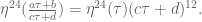
To see why the linking number is at all related to the eta function, one uses Jacobi’s identity 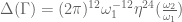


[Another proof equating the linking number to an alternate, more topological, definition of the Radamacher number is also sketched out in Étienne’s proceedings article.]
The second remarkable theorem about these modular knots is that the knot types (or more precisely, isotopy classes) of the modular knots coincide exactly with the knot types of the Lorenz attractor periodic orbits! Similarly for the link types between knots. This unexpected connection between dynamics and number theory arises from two key facts. The first, which is relatively easy, is that the modular flow contains inside it an invariant set which is equivalent to the Lorenz template briefly mentioned earlier; this set can be constructed explicitly by flowing out from the regular hexagonal and equilateral lattices in the unstable directions. The second, which is trickier, is to show that any knot in the larger moduli space M can be continuously deformed onto this template (and furthermore, any link of knots can be continuously deformed onto this template). This was not proved in Étienne’s talk, but there were several very nice computer animations which displayed this deformation quite convincingly.
There appear to be several further connections between the modular flow and the Lorenz flow which is work in progress, but this was not detailed in the talk.
Étienne closed by commenting on the importance on communicating mathematics effectively not just to other mathematicians in one’s field or on other fields, but also to non-mathematicians; for instance, Jos Leys, who created all the computer animations for the talk, is a mechanical engineer with a keen interest in mathematics. He ended with two supporting quotes from David Hilbert (at an ICM over a century earlier):
“A mathematical theory is not to be considered complete unless you made it so clear that you can explain it to the man in the street.”
“For what is clear and easily comprehended attracts, and the complicated repels us.”
Étienne remarked that Hilbert’s second quote is a particularly succinct explanation of why he loves mathematics (and it is why I do too).
[Update, Aug 4: link corrected.]

11 comments
Comments feed for this article
3 August, 2007 at 12:44 pm
bk
Dr Tao,
Can you give more talks on PDE?
3 August, 2007 at 4:00 pm
Top Posts « WordPress.com
[…] 2006 ICM: Étienne Ghys, “Knots and dynamics” Almost a year ago today, I was in Madrid attending the 2006 International Congress of Mathematicians (ICM). One of the […] […]
3 August, 2007 at 4:18 pm
A couple of links! « Entertaining Research
[…] Terry Tao on a talk that he attended (nearly an year ago) on knots and dynamics. […]
3 August, 2007 at 10:47 pm
Doug
Hi Terrence,
This is a fascinating thread [!] that may relate to other ideas?
E Ghys slides of “Knots and dynamics” discusses
– knots with orbit periodicity
— [nearly circular ellipse if planar?, helix if trajectory curve?],
– “helicity as asymptotic linking number” or
— “a topological invariant”,
– torus — “suspension” related to helicity.
Perhaps there exists a relation with:
a – Urs Wiedemann [CERN], ‘Jet quenching in string theory and heavy ion collisions’ emphasizing “our task: find catenary”, slide 38/38, Strings 07.
— Euler related the catenary to the catenoid,
— the catenoid is in isometry with the helicoid,
— the helix is an elliptical and trajectory curve forming a virtual helicoid.
b – DM Stump, AR Champneys, GHM van der Heijden, ‘The torsional buckling and writhing of a simply supported rod hanging under gravity’, “… outer catenary-like solution … modulated helix-like spiral with period …”.
International Journal of Solids and Structures
Volume 38, Issue 5, February 2001, Pages 795-813
c – David Hestenes, ‘The Kinematic Origin of Complex Wave Functions’, “… wave function describes electron … Zitterwebegung interaction …”.
d – supercoiling helices of ionic, nucleic and amino acids
– may help explain bioelectromagnetism.
[compare Ghys slide 19/40 with images of DNA, RNA, protein helices; rope and cable wiring and images of helices in space by NASA]
Note:
The helix appears to be ubiquitous at many different scales.
The above structures may have similarity with helical wired solenoids.
– an iron core solenoid may have a magnetic field several hundred times that of an equivalent air solenoid.
[image in GSU Hyperphysics on google]
Speculation:
Pehaps gravity may be a solenoid like force [partial, virtual?] as is electromagnetism in many cases?
– EM waves (helical) may form vacuum solenoids?
– Planetary and star orbits are nearly circular ellipses when sun or galactic nucleus held stationary with helical angle equal zero;
when sun or galactic nucleus in motion, helical angle greater than zero?
– The weak and strong forces under SU(3) x SU(2) x U(1) are virtually transformed into electromagetism?
The torus may relate to the Monster symmetry with “folded” [doughnut] possible rather than only “broken” symmetry?
4 August, 2007 at 9:13 am
amazeen
The link to moduli space is wrong. It sends you to the wikipedia page on discriminants.
4 August, 2007 at 9:14 am
In case you thought I had given up on knot theory « Mumble Mumble…
[…] blogger Terrance Tao has a really cool post summarizing a talk from the 2006 ICE about the marriage of knot theory and dynamical systems. Specifically, he talks about the use of limits of knots (whatever that means…) as a way of […]
4 August, 2007 at 9:51 am
Terence Tao
Dear amazeen,
Thank you for the correction!
5 August, 2007 at 6:53 am
GVietMath Thế nào là một lý thuyết toán học tốt? «
[…] cho ra Trích từ một bài viết gần đây của Terence […]
8 August, 2007 at 2:32 pm
Carnival of Mathematics XIV « Vlorbik on Math Ed
[…] Category Theory), and Questions About Modules (by John Baez in The n-Category Cafe). Also Terry Tao reports on ICM 2006, where he seems to have won some sort of […]
15 September, 2009 at 11:19 am
Anonymous
All the videos of the congress, including Étienne Ghys talk, are available at http://www.icm2006.org/video/ .
12 June, 2017 at 1:18 am
Some notes on Lorenz flow – Math for everyone
[…] In 2006 Ghys discovered the extraordinary fact that the set of periodic orbits of the Lorenz equations is identical to that of the geodesic flow on the unit tangent bundle to the modular surface http://www.math.tifr.res.in/~tali/research/research_statement.pdf https://terrytao.wordpress.com/2007/08/03/2006-icm-etienne-ghys-knots-and-dynamics/ […]