In the third Marker lecture, I would like to discuss the recent progress, particularly by Goldston, Pintz, and Yıldırım, on finding small gaps  between consecutive primes. (See also the surveys by Goldston-Pintz-Yıldırım, by Green, and by Soundararajan on the subject; the material here is based to some extent on these prior surveys.)
The twin prime conjecture can be rephrased as the assertion that attains the value of 2 infinitely often, where  are the primes. As discussed in previous lectures, this conjecture remains out of reach at present, at least with the techniques centred around counting solutions to linear equations in primes. However, there is another direction to pursue towards the twin prime conjecture which has shown significant progress recently (though, again, there appears to be a significant difficulty in pushing it all the way to the full conjecture). This is to try to show that is unexpectedly small for many n. Let us make this a bit more quantitative by posing the following question:
Question. Let N be a large number. What is the smallest value of , where  is a prime between N and 2N?
The twin prime conjecture (or more precisely, the quantitative form of this conjecture coming from the prime tuples conjecture) would assert that the answer to this question is 2 for all sufficiently large N.
There are various ways to get upper bounds on this question. For instance, from Bertrand’s postulate (which can be proven by elementary means) we know that  for all
  . The prime number theorem asserts that
  , which gives
  ; using various non-trivial facts known about the zeroes of the zeta function, one can improve this to
  for various c (the best value of c known unconditionally is
  , a result of Baker, Harman, and Pintz). The Riemann hypothesis gives a significantly more precise asymptotic formula for , which ultimately leads to the bound
  . These bounds hold for all n in the given range, and so in fact bound the largest value of , not just the smallest. As far as I know, the
  bound for the largest prime gap has not been improved even after one assumes the Riemann hypothesis, though this gap is generally expected to be much smaller than this. (In particular, the old conjecture that there always exists at least one prime between two consecutive square numbers remains open, even assuming RH. Cramér conjectured a bound of
  , though it is possible that the constant 1 here may need to be revised upwards to
  where
where  is the Euler-Mascheroni constant, see this paper of Granville for details.) In the converse direction, the best result is due to Rankin, who showed the somewhat unusual bound

for some n and some absolute constant  (in fact one can take c arbitrarily close to
  ). Remarkably, this type of right-hand side appears to be a genuine limit of what current methods can achieve (Paul Erdős in fact offered $10,000 to anyone who could improve the rate of growth of the right-hand side in N).
But for the smallest value of , much more is known. The prime number theorem already tells us that there are  primes between N and 2N, so from the pigeonhole principle we have
 (1)
(1)
for some n.
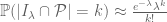
This bound should not be sharp, since this would imply that the primes are almost equally spaced by  , which is suspiciously regular behaviour for a sequence as irregular as the primes. To get some intuition as to what to expect, we turn to random models of the primes. In particular, we begin with Cramér’s random model for the primes, which asserts that the primes between N and 2N behave as if each integer in this range had an independent chance of about
  of being prime. Standard probability theory then shows that the primes are distributed like a Poisson process of intensity . In particular, if one takes an random interval
  in
in ![{}[N,2N]](https://s0.wp.com/latex.php?latex=%7B%7D%5BN%2C2N%5D&bg=ffffff&fg=545454&s=0&c=20201002) of length
of length  for some
  , the number of primes
  that captures is expected to behave like a Poisson random variable of mean
  ; in other words, we expect
 (2)
(2)
for  . (In contrast, the prime number theorem only gives the much weaker statement
  .)
.)
Now, as discussed in previous lectures, Cramér’s random model is not a completely accurate model for the primes, because it does not reflect the fact that primes very strongly favour the odd numbers, the numbers coprime to 3, and so forth. However, it turns out that even after one corrects for these local irregularities, the predicted Poisson random variable behaviour (2) does not change significantly for any fixed (e.g. a Poisson process of intensity  on the odd numbers looks much the same as a Poisson process of intensity on the natural numbers, when viewed at scales comparable to ). This computation was worked out fully by Gallagher as a rigorous consequence of the Hardy-Littlewood prime tuples conjecture. (On the other hand, these corrections to the Cramér model do disrupt (2) for very large values of ; see this paper of Soundararajan for more discussion.)
Applying (2) for small values of (but still independent of N), we see that intervals of length are still expected to contain two or more primes with non-zero probability, which in particular would imply that  for at least one value of n. So one path to creating small gaps between primes is to show that can exceed 1 for as small a value of as one can manage.
One approach to this proceeds by controlling the second moment
 ; (3)
; (3)
the heuristic (2) predicts that this second moment should be  (reflecting the fact that the Poisson distribution has both mean and variance equal to ). On the other hand, the prime number theorem gives the first moment estimate . Also, if never exceeds 1, then the first and second moments are equal. Thus if one could get the right bound for the second moment, one would be able to show that is possible for arbitrarily small .
Second moments such as (3) are very amenable to tools from Fourier analysis or complex analysis; applying such tools, we soon see that (3) can be re-expressed easily in terms of zeroes to the Riemann zeta function, and one can use various standard facts (or hypotheses) about these zeroes to gain enough control on (3) to obtain non-trivial improvements to (1). This approach was pursued by many mathematicians including Hardy-Littlewood, Rankin, Erdős, and Bombieri-Davenport; leading to non-trivial unconditional results for any  , but it seems difficult to push the method much beyond this. It was later shown by Goldston and Montgomery that the correct asymptotic for (3) is essentially equivalent to the Riemann hypothesis combined with a certain statement on pair correlations between zeroes, and thus well out of reach of current technology.
Another method, introduced by Maier, is based on finding some (rare) intervals of numbers of length for some moderately large which contain significantly more primes than average value of ; if for instance one can find such an interval with over  primes in it, then from the pigeonhole principle one must be able to find a prime gap of size at most
  . The ability to do this stems from the remarkable and unintuitive fact that the regularly distributed nature of primes in long arithmetic progressions, together with the tendency of primes to avoid certain residue classes, forces the primes to be irregularly distributed in short intervals. This phenomenon (which has now been systematically studied as an “uncertainty principle” for equidistribution by Granville and Soundararajan), is related to the following curious failure of naive probabilistic heuristics to correctly predict the prime number theorem. Indeed, consider the question of asking how likely it is that a randomly chosen number n between N and 2N is to be prime. Well, n will have about a
  chance of being coprime to 2, a
  chance of being coprime to 3, and so forth; the Chinese remainder theorem also suggests that these events behave independently. Thus one might expect that the probability would be something like
 .
.
We then invoke Mertens’ theorem, which provides the asymptotic
 . (4)
. (4)
But this is off by a factor of  from what the prime number theorem says the true probability of being prime is, which is
  . This discrepancy reflects the difficulty in cutting off the product in primes (4) at the right place (for instance, the sieve of Eratosthenes suggests that one might want to cut off at
  instead) and I might discuss this topic further in a future blog post. At any rate, this
  discrepancy can be exploited to find intervals with an above-average number of primes by a “first moment” argument (known as the Maier matrix method) that we sketch as follows. Let w be a moderately large number, and let W be the product of all the primes less than w. If we pick a random number n between N and 2N, then as mentioned before, the prime number theorem says that this number will be prime with probability about
  . But if in addition we know that the number is coprime to W, then by the prime number theorem in arithmetic progressions this information boosts the probability of being prime to about
  , which by (4) is about
  .
.
Now we restrict attention to numbers n which are equal to a mod W for some  . By the prime number theorem, about
  of the a are prime and thus coprime to W. Combining this with the previous discussion, we see that the total probability that such a number n is prime is about
  .
.
On the other hand, the set of numbers n which are equal to a mod W for some is given by a sequence of intervals of length w. By the pigeonhole principle, we must therefore have an interval of length w on which the density of primes is at least  – which is greater than the expected density by a factor of .
One can make the above arguments rigorous for certain ranges of interval length, and by combining this with the pigeonhole principle one can eventually improve (1) by a factor of :
 .
.
This is better than the bound of  obtained by the second moment method, but on the other hand the latter method establishes that a positive proportion of primes have small gaps; Maier’s method, by its very nature, is restricted to a very sparse set of primes (note that w is much smaller than W).
In a series of papers, Goldston and Yıldırım improved the numerical constants in these results by a variety of methods including those mentioned above, as well as replacing some of the reliance on information on zeroes of the zeta function with tools from sieve theory instead. To oversimplify substantially, the latter idea is to try to control the set of primes  in terms of a larger set
  of almost primes – numbers with few prime factors. (Strictly speaking, one does not actually work with a set of almost primes, but rather with a weight function or sieve which is large on almost primes and small for non-almost primes, but let us ignore this important technical detail to simplify the exposition.) For instance, to control the second moment , one can take advantage of the Cauchy-Schwarz inequality

The denominator on the right-hand side involves only almost primes and can be computed easily by sieve theory methods. The numerator involves primes, but only one prime at a time; note that this quantity is roughly counting the set of pairs  where p is prime, q is almost prime, and p and q differ by at most . This is in contrast to the left-hand side, which is counting pairs p, q that are both prime and differ by at most . We do not know how to use sieve theory to count the latter type of pattern (involving more than one prime); but sieve theory is perfectly capable of counting the former type of pattern, so long as we understand the distribution of primes in relatively sparse arithmetic progressions. The standard tool for this is the Bombieri-Vinogradov theorem, which roughly speaking asserts that the primes from N to 2N are well distributed in “most” residue classes q, as long as q stays significantly smaller than ; it can be viewed as an averaged version of the generalised Riemann hypothesis that can be proven unconditionally. (The key point here is that while it is possible for the primes to be irregular with respect to a few such small moduli, the “orthogonality” of these moduli with respect to each other makes it impossible for the primes to be simultaneously irregular with respect to many of these moduli at once. I may comment more on this topic in a future post.) Using such tools, various improvements to (1) were established. Finally, in 2005, in a series of papers by Goldston, Pintz, and Yıldırım, it was shown that
 (5)
(5)
held for some n and any (provided N was large enough depending on ), or equivalently that  ; this was later improved further, to
  . Assuming a strong version of the Bombieri-Vinogradov theorem (in which q is allowed now to get close to N rather than to ), known as the Elliott-Halberstam conjecture), this was improved further to the striking result

thus there are infinitely many pairs of primes which differ by at most 16. This is a remarkable “near miss” to the twin prime conjecture, though it seems clear that substantial new ideas would be needed to reduce 16 all the way to 2.
Let’s now discuss some of the ideas involved. As with the previous arguments, the key idea is to find groups of integers which tend to contain more primes than average. Suppose for instance one could find a certain random distribution of integers n where n, n+2, and n+6 each had a probability strictly greater than 1/3 of being prime. (We choose these separations for our discussion because it is not possible to make three large prime numbers bunch up any closer than this; for instance, n, n+2, n+4 cannot be all be prime for  , since at least one of these numbers must be divisible by 3.) By linearity of expectation, we thus see that the expected number of primes in the set
  exceeds 1; thus, with positive probability, there will be at least two primes in this set, which then necessarily differ by at most 6.
Now, of course, the prime number theorem tells us that for n chosen uniformly at random from N to 2N, the probability that n, n+2, or n+6 are prime is only about . So for this type of strategy to work, one would have to pick a highly non-uniform distribution for n, in which n, n+2, and n+6 are already close to being prime already. The extreme choice would be to pick n uniformly among all choices for which n, n+2, and n+6 are simultaneously prime, but we of course don’t even know that any such primes exist (this is strictly harder than the twin prime conjecture!) But what we can do instead is pick n uniformly among all choices such that n, n+2, and n+6 are almost prime (where we shall be vague for now about what “almost prime” means). Thanks to sieve theory, we can assert the existence of many numbers n of this form, and get a good count as to how many there are. Also, since the primes have positive density inside the almost primes, it is quite reasonable that the conditional probabilities
 ,
,
 ,
,
 ,
,
are large. Indeed, using sieve theory techniques (and the Bombieri-Vinogradov theorem), we can bound each of these probabilities from below by a positive constant (plus a o(1) error). Unfortunately, even if we optimise the sieve that produces the almost primes, this constant is too small (typically one gets numbers of the order of 1/20 or so, rather than 1/3). Assuming the Elliot-Halberstam conjecture (which allows us to raise the level of sieving substantially) yields a significant improvement, but one that still falls short of the desired goal. One can of course also add more numbers to the mix than just  , e.g. looking at those n for which
  are simultaneously almost prime, for some suitably chosen
  ; on the one hand this lowers the threshold of probability (currently at 1/3) that one needs to obtain, but unfortunately this is more than canceled out by the multidimensional sieving one needs to do when restricting all of these numbers to be almost prime.
To get around this, a new idea was introduced: instead of requiring numbers such as n, n+2, and n+6 to separately be almost prime, ask instead for the product n(n+2)(n+6) to be almost prime (for a somewhat more relaxed notion of “almost prime”). This turns out to be more efficient, as it lowers the number of summations involved in the sieve. One has to carefully select how one defines almost prime here (it is roughly like asking for the product  to have at most
  prime factors, with the o(k) factor being remarkably crucial to the delicate analysis); but to cut a long story short, one can establish probability bounds of the form
 (6)
(6)
for all  and some absolute constant
  . [More formally, one needs to compute sums such as
  , where
  is the von Mangoldt function and
  is a Selberg sieve-type approximation to that function.]
As soon as one assumes any non-trivial portion of the Elliott-Halberstam conjecture, the quantity c in the above inequality can be made to exceed 1 (for k large enough), leading to the conclusion that there exist infinitely many bounded prime gaps,  ; pushing the machinery to their limit (taking
  to be the first six primes larger than 6), one obtains the bound of 16. But without this conjecture, and just using Bombieri-Vinogradov, then after optimising everything in sight, one can get c arbitrarily close to 1, but not quite exceeding 1. To compensate for this, the authors also started looking at the nearby numbers n+h where h was not equal to . Here, of course, there is no particularly good reason for n+h to be prime, since it is not involved as a factor to the almost prime quantity
  ; but one can show that, for generic values of h, one has

for some  (there is an additional singular series factor involving the prime factors of
  which can be easily dealt with, that I am suppressing here.) Thus, for any , we expect (from linearity of expectation) that for almost prime, the expected number of
  (including the k values ) for which n+h is prime is at least
 .
.
Since we can make c arbitrarily close to 1, the extra term  can push this expectation to exceed 1 for any choice of , and this leads to the desired bound (5) for any . (The subsequent improvement to (5) proceeds by enlarging k substantially, and by a preliminary sieving of the small primes, but we will not discuss these technical details here.)
It is tempting to continue to optimise these methods to improve the various constants, and I would imagine that the bound of 16, in particular, can be lowered somewhat (still assuming the Elliott-Halberstam conjecture). But there seems to be a significant obstacle to pushing things all the way to 2. Indeed, the parity problem tells us that for any reasonable definition of “almost prime” which is amenable to sieve theory, the primes themselves can have density at most 1/2 in these almost primes. Since we need the density to exceed 1/k in order for the above argument to work, it is necessary to play with at least three numbers (e.g. n, n+2, n+6), which forces the bound on the prime gaps to be at least 6. (Indeed, this bound has been obtained for semiprimes – which are subject to the same parity problem restriction as primes, but are slightly better distributed – by Goldston, Graham, Pintz, and Yıldırım.) But it may be that a combination of these techniques with some substantially new ideas may push things even further.


14 comments
Comments feed for this article
20 November, 2008 at 11:51 am
Emmanuel Kowalski
That’s a very nice discussion!
Maybe I can also direct the interested reader to my own survey (a Bourbaki seminar report), in particular to the last section which contains more discussion of the obstacles and possibilities in trying to work beyond the Bombieri-Vinogradov theorem — there are results of Fouvry, Bombieri, Friedlander, Iwaniec that go beyond the bound for moduli of primes in arithmetic progressions, although they are not of the right type of results to get bounded gaps between primes.
Also it may be of interest to mention that one can generalize fairly easily Gallagher’s conditional argument leading to a Poisson distribution to show that — under the same assumption — the number of (say) twin primes between and
and  should also asymptotically be Poisson distributed (with parameter
  where
where  is the twin-prime constant).
21 November, 2008 at 8:18 pm
Terence Tao
Dear Emmanuel,
Thanks for the reference and the comments!
15 December, 2008 at 4:47 am
mike
do you have any information on how the twin prime constant was derived?
30 July, 2009 at 11:13 pm
peter acquaah
you are simply great!
In fact, I think you should check this idea.
http://www.geocities.com/SoHo/Exhibit/8033/pgtow/pgtow.html
I was working on something like that and I agree with the author’s work.
Keep it up Tao.
16 November, 2011 at 3:00 am
EGME
Dear Terry,
Consider the following: let t be a generator( of a twin prime pair) if 6t+1, 6t-1 are primes. Let f be a sequence, for example, the sequence {5p}, where p is a prime, and let g be the largest gap between generators contained in f up to f(n), where f(n) is a generator contained in f. I speculate the following. Between f(n) and f(n+2g)there is another element of f which is a generator. How might one appproach this problem probabilistically, for example, show that the probability of finding such a generator is greater than 0?
20 November, 2011 at 10:44 pm
EGME
More precisely,
Let f(i)={5*p(i)} be a sequence where p(i) is the i-th prime. Suppose that that there is a maximum gap, for i<=n, of g, meaning, that for any for any m<=n
{ f(p(m+1)),…f(p(m+g+1)) } has as at least one twin prime generator, and for any some q20, there is a generator in {f(p(n)),…,f(p(n+2g))}. I have checked this up to n=700 meg. Moreover, between i=100 million and i=700 million, there is no increase in max gap size. max gap increases sligtly from i=700 meg to 800 meg, as expected from observing the behavior in the first 70 meg entries..
29 November, 2011 at 10:20 pm
petequinn
Prof Tao, in this article you wrote “This discrepancy reflects the difficulty in cutting off the product in primes (4) at the right place (for instance, the sieve of Eratosthenes suggests that one might want to cut off at instead) and I might discuss this topic further in a future blog post. ” Did you ever elaborate on this issue in a later article? I’m interested to explore this further.
Thanks,
Pete
28 December, 2011 at 9:29 pm
petequinn
Professor Tao,
the link to Granville’s paper above, referred here:
“Cramér conjectured a bound of —, though it is possible that the constant 1 here may need to be revised upwards to — where is the Euler-Mascheroni constant, see this paper of Granville for details.)”
appears to be dead. Is it possible to re-identify the paper you’d linked? I’m very interested to explore this aspect in a bit more detail if possible.
Best for the holidays,
Pete
28 December, 2011 at 9:30 pm
petequinn
Apologies, ignore the last. I see the paper citation at the referred link, thanks
Pete
23 May, 2013 at 6:18 am
The Beauty of Bounded Gaps | sladisworld
[…] concerning the remainders obtained after division by many different integers. From this (following a path laid out by Goldston, Pintz, and Yıldırım, the last people to make any progress on prime gaps) he can show that the prime numbers look random […]
30 December, 2014 at 7:37 pm
George Sands
I am not a mathematician though I work at a high level in a closely related field. I am trying to be helpful in my comments here. I think I know enough to know, but if I am “trolled” or “facebooked” in any way, I will request that my comments be deleted. I believe math should be kind and collegial, only. Latex problems are a function of the format.
Let us consider the Twin Prime Conjecture, and suppose that it is false for purposes of this post.
This means that there is a prime number, , such that the pair
  has the property that
  but that there is no larger such pair of primes.
Call the infinite set of primes that excludes the first N primes. One can then consider the set
  , which is generated by sum, products, and differences of elements of
  . If one adds the number 1 to the set
  and then generates a ring, it turns out that the resultant ring is all the integers. This follows from the fact that if
  are relatively prime integers, then there are integers
  such that
  . The reader should check this. It is a well-known result we learned in kindergarten Number Theory, as a friend is fond of saying (a funny friend, meant humorously).
Since the ring is the integers, we know that 2 is the difference of two “generators” — elements such that
  . The question on which this post focuses, and there are “deep” reasons for starting with this suggestion to others to look at the problem in this way, is what “shape” can c and d take, without generating a contradiction with our starting point: suppose that the Twin Prime Conjecture is false. Our hope is to generate contradictions.
1. We know that c and d cannot be prime since this would create a contradiction.
2. If c and d are minimal in the sense that we have no smaller pair, in the sense of , S is minimal, can either c or d be a prime number?
I suggest that the assembled readers of the blog can prove relatively quickly that neither c or d can be prime.
3. If c and d are minimal in the sense that we have no smaller pair, in the sense of , S is minimal, it is apparent that c and d must be coprime.
4. Furthermore, I think it is the case that if c is the product of several prime numbers (greater than of course) and so is d, and c and d are minimal in the sense defined above, then we know that the exponents of the prime numbers that factor c, and the exponents of the prime numbers that factor d, cannot
  have a common divisor. For example, we cannot have
  and
and  .
.
Why? This is left to the reader to verify.
Of the steps laid out so far, step 2 is by far the hardest, but very attainable. To motivate ideas, take and
and  . This is a convenient example for seeing how to prove step 2. It is sufficently “rich” and sufficiently “simple.” That, I think, should be enough of a hint for many readers.
One readers post answers to all of these parts, I will post the next steps, along with associated “suggestions” or “hints.” The beginning mathematician will want to verify that the ring generated by and 1 is in fact the integers.
30 December, 2014 at 7:46 pm
George Sands
Regarding step 2, I meant to include this. Start with the case where one supposes and
and  . Exclude from consideration, at this juncture, d that factor into multiple primes (all greater than of course
  as we have defined
  .
.
Hope that helps make step 2 a bit more reachable.
31 December, 2014 at 11:33 am
Anonymous
Question. Let N be a large number. What is the smallest value of p_{n+1}-p_n, where p_n is a prime between N and 2N?
To answer this question, the Riemann Hypothesis is not that helpful. In other words, one cannot do particularly well with assuming RH is true. Why? That’s the subject of a paper itself.
What is instead needed to do better is to understand the distribution function for the zeros of the function along the critical line, whether or not there are zeros elsewhere in the critical strip. Why? Well consider Riemann’s original formula for the function
  along the line
  (the critical line — refer the reader to the original paper, which is translated into English in various papers — for that function). In the integrand is a function which Riemann calls
  .
.  . Think about it for a while.
Maybe I’ve said too much, given the Clay Prize. However, I think people will have enough trouble seeing why they should focus attention on JUST the zeros on the critical line, Riemann’s formula for , and why the function
  relates to the distribution of zeros along the line as well as to the prime numbers themselves. It shouldn’t be THAT hard, but sometimes it is not that easy to see either.
8 November, 2016 at 6:35 am
A huge discovery about prime numbers – Emmanuel A. Otchere's Blog
[…] concerning the remainders obtained after division by many different integers. From this (following a path laid out by Goldston, Pintz, and Yıldırım, the last people to make any progress on prime gaps) he can show that the prime numbers look random […]