
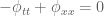
As is well known, the linear one-dimensional wave equation
where 

for some arbitrary (smooth) functions 
When one moves from linear wave equations to nonlinear wave equations, then in general one does not expect to have a closed-form solution such as (2). So I was pleasantly surprised recently while playing with the nonlinear wave equation
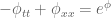
to discover that this equation can also be explicitly solved in closed form. (I hope to explain why I was interested in (3) in the first place in a later post.)
A posteriori, I now know the reason for this explicit solvability; (3) is the limiting case 

which (after applying the simple transformation 
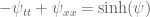
(a close cousin of the more famous sine-Gordon equation 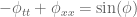
[The computations do seem to be very classical, though, and thus presumably already in the literature; if anyone knows of a place where the solvability of (3) is discussed, I would be very happy to learn of it.] [Update, Jan 22: Patrick Dorey has pointed out that (3) is, indeed, extremely classical; it is known as Liouville’s equation and was solved by Liouville in J. Math. Pure et Appl. vol 18 (1853), 71-74, with essentially the same solution as presented here.]
— Symmetries of (3) —
To simplify the discussion let us ignore all issues of regularity, division by zero, taking square roots and logarithms of negative numbers, etc., and proceed for now in a purely formal fashion, pretending that all functions are smooth and lie in the domain of whatever algebraic operations are being performed. (It is not too difficult to go back after the fact and justify these formal computations, but I do not wish to focus on that aspect of the problem here.)
Although not strictly necessary for solving the equation (3), I find it convenient to bear in mind the various symmetries that (3) enjoys, as this provides a useful “reality check” to guard against errors (e.g. arriving at a class of solutions which is not invariant under the symmetries of the original equation). These symmetries are also useful to normalise various special families of solutions.
One easily sees that solutions to (3) are invariant under spacetime translations

and also spacetime reflections
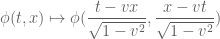
Being relativistic, the equation is also invariant under Lorentz transformations
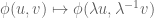
Finally, one has the scaling symmetry

— Solution to (3) —
Henceforth 
thus
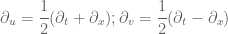
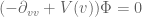
and (3) becomes

The various symmetries (4)-(7) can of course be rephrased in terms of null coordinates in a straightforward manner. The Lorentz symmetry (6) simplifies particularly nicely in null coordinates, to
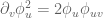
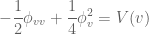
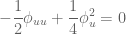
Motivated by the general theory of stress-energy tensors of relativistic wave equations (of which (3) is a very simple example), we now look at the null energy densities 


(One can also see this from the explicit solution (2).)
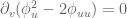
The above transport law isn’t quite true for the nonlinear wave equation, of course, but we can hope to get some usable substitute. Let us just look at the first null energy 


and thus we have the pointwise conservation law
which implies that

for some function 
for some function 
For any fixed v, (11) is a nonlinear ODE in u. To solve it, we can first look at the homogeneous ODE
Undergraduate ODE methods (e.g. separation of variables, after substituting 


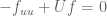
and hence (11) becomes

thus 

we thus have
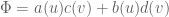
for some functions c, d (which one easily verifies to be smooth, since 
and hence (by linear independence of a, b) c, d must be solutions to the ODE

This would be a good time to pause and see whether our implications are reversible, i.e. whether any

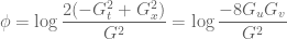
one soon sees that (10) is equivalent to

If we then insert the ansatz (14), we soon reformulate the above equation as

It is at this time that one should remember the classical fact that if a, u are two solutions to the ODE (11), then the Wronskian 

Theorem. A smooth function
,
for some constants
multiplying to
.
Note that one can generate solutions to the Wronskian equation 
This is not the only way to express solutions. Factoring a(u)d(v) (say) from (12), we see that 


and so we see that
for some solution G to the free wave equation, and conversely every expression of the form (16) can be verified to solve (1) (since 

to (1), where f and g are arbitrary functions (recall that we are neglecting issues such as whether the quotient and the logarithm are well-defined).
I, for one, would not have expected the solution to take this form. But it is instructive to check that (17) does at least respect all the symmetries (4)-(7).
— Some special solutions —
If we set U=V=0, then a,b,c,d are linear functions, and so 


To express this solution in the form (17), one can take 

We can also look at what happens when 


To express this solution in the form (17), one can take for instance 

One can of course push around (18), (19) by the symmetries (4)-(7) to generate a few more special solutions.

30 comments
Comments feed for this article
22 January, 2009 at 2:33 pm
Anonymous
Nice post! A very low-level question: are there simple cases in which non-linear heat equations can be solved in closed-form?
22 January, 2009 at 3:36 pm
Terence Tao
Well, I know that the viscid Burgers equation can be solved explicitly by the Cole-Hopf transformation
  to the heat equation
  , and scalar harmonic map heat flow equations such as
  can be similarly solved by a change of coordinates to trivialise the target (in this case, one sets
  to obtain the linear heat equation
  ). There are probably a few other examples too.
Now that I have learned the provenance of the equation in the post as Liouville’s theorem (within two hours of posting it!) I wonder whether it could ever be possible to “Google” for an equation, without knowing its name, to find out the existing literature on it (much as the online encyclopedia of integer sequences does for sequences). One has the DispersiveWiki, of course, but this equation was not listed there (though I’ve fixed that now…). In the meantime, it seems that asking readers through a blog is one of the more efficient ways to answer these sorts of questions.
22 January, 2009 at 4:03 pm
Anonymous
Incidentally – since the heat equation is non-relativistic, and since Lorentz symmetry is an important piece of the puzzle in your post – is there a relativistic form of the heat equation that is somehow more natural?
22 January, 2009 at 7:09 pm
Jake K.
There’s a couple typos.
* Equation (10) isn’t actually labeled as such
* After “this density obeys the transfer equation”, in the displayed math there’s a “phi_uv” that should be “phi_{uv}” [Corrected, thanks – T.]
23 January, 2009 at 7:36 am
The Art of Finding General Solutions « Teaching
[…] to obtain general solutions, and that there is no universally effective algorithm to follow. This post, appearing yesterday on Prof. Terence Tao’s blog, reveals how one of today’s very best […]
23 January, 2009 at 7:39 am
M. E. Irizarry-Gelpí
This is a very illuminating post. Thanks for sharing this result.
23 January, 2009 at 7:45 am
user
I too wish there was a large searchable database of mathematical expressions, but I have never seen anyone actually implement one. We should try to get someone at Google to spend their “innovation time off” and implement such a search feature. Paired with a database such as MathSciNet (which contains lots of expressions in TeX-format, which is a lot easier to parse to a tree-form compared to OCRed text) it would be pretty awesome.
As of now, we are left with trying to figuring out how the OCR/text conversion process will botch the mathematical expressions. In this case, it actually worked: searching for uxx utt eu (try it on Google Book search: http://books.google.com/books?q=utt+uxx+eu ) gives the correct answer (searching for is not as easy though, but it can work if the text was not OCRed). Always easy in hindsight…
23 January, 2009 at 8:26 am
maglev
Dear Terry,
The wave equation, which was used e.g., for determining the speed of light, is an approximation of a discrete version. Does the discrete wave equation also have a closed form solution of (2) type?
23 January, 2009 at 7:49 pm
Terence Tao
Dear anonymous: I have occasionally seen relativistic versions of the heat equation proposed, for instance by Brenier, but I do not know how well grounded their physical derivations are; presumably there must be some literature on relativistic thermodynamics and statistical mechanics, but this is somewhat outside of my own area of expertise. (The Schrodinger equation, which is superficially similar in appearance to the heat equation, has relativistic analogues, such as the Klein-Gordon or Dirac equations, but this does not seem to shed any light as to what the relativistic heat equation should be.)
Dear user: that’s a nice trick (searching for a mangled version of the equation); I’ll bear it in mind next time I come up against this sort of issue.
Dear maglev: the discrete linear wave equation has essentially the same solution (2) as its continuous counterpart. There appear to be discrete analogues of the Liouville equation in the literature (it is quite common for exactly solvable integrable systems to have discrete analogues that are also exactly solvable), but I do not know much about them as yet.
24 January, 2009 at 7:12 am
gambit
Dear Terry,
You are right, however, if one considers the classical
{\ddot u}_n = u_{n+1} – 2u_n + u_{n-1}, n \in Z, with the initial conditions u_n (t=0)=\delta_{n0}, {\dot u}_n (t=0)=0, then the solution u_n (t) = J_{2n} (2t) is dispersive.
24 January, 2009 at 9:07 am
The high exponent limit $p to infty$ for the one-dimensional nonlinear wave equation « What’s new
[…] In the remainder of this post I would like to describe the strategy of proof and one of the key a priori bounds needed. I also want to point out the connection to Liouville’s equation, which was discussed in the previous post. […]
24 January, 2009 at 3:14 pm
Th%
Hello, Professor Tao. I remember equation (3) was called Liouville equation when I learned how to find its solutions using Backlund transformations 20 years ago. These transformations apply solutions of Liouville to solutions of the wave equations and back. I think Liouville actually solved the elliptic equation in this way. My interest was that superposition principle of the linear equation was tranformed to a non linear combination law, and I seeked to understand what happens in the quantum case. I believe this method is essentially equivalent to yours, at least with the same result (17). But I like your presentation of this result.
25 January, 2009 at 3:35 am
hydrobates
Dear Terry,
I just wanted to make a comment on the difficult subject of relativistic generalizations of the heat equation, which relates to the wider question of relativistic generalizations of the Navier-Stokes equations. A basic problem is that the infinite propagation speed associated with diffusion is not compatible with the limitation of speeds by the speed of light in (special) relativity. A relativistic equation for a viscous fluid should naturally turn out to be hyperbolic rather than parabolic. The attempt to derive equations of this type from kinetic theory succeeds in the sense that the existence of a reasonable system is OK but there is a huge non-uniqueness. As a source of a lot more information on this topic than I possess I recommend the review article by Ingo Muller in the online journal Living Reviews in Relativity.
25 January, 2009 at 1:16 pm
IM
Dear Terry,
Following up from my earlier questions, then (as Anonymous): is there a sense in which the Dirac or Klein-Gordon equations are mathematically “nicer” than the Schrodinger equation? And if so, might there be analogues of this for the heat equation/ Navier-Stokes equation?
I guess what I’m asking (from, as is probably clear, a position of almost total ignorance) is whether an oblique approach, of taking the nonrelativistic limit of a relativistic equation, is ever a better way of attacking the nonrelativistic equation itself.
26 January, 2009 at 6:21 am
McGuigan
The Lagrangian associated with the Liouville equation is
important in the study of 1+1 dimensional quantum gravity
and strings. For example:
Quantum Geometry of Bosonic Strings.
Alexander M. Polyakov .
Published in Phys.Lett.B103:207-210,1981
Liouville field theory: A Decade after the revolution.
Yu Nakayama (Tokyo U.) . UT-04-02, Jan 2004. 261pp.
Published in Int.J.Mod.Phys.A19:2771-2930,2004.
e-Print: hep-th/0402009
Distler and Kawai: Conformal Field Theory And 2d Quantum Gravity Or Who’s Afraid Of Joseph Liouville?Nucl.Phys.B321:509,1989 [
If one multiples both sides of the equation by e^{-phi}
and quantizes this as in the above references would this
be an approach to quantized wave maps, simpler than the 2+1 quantum gravity connnection discussed previously.?
26 January, 2009 at 7:26 am
dynamic stripes
Deer maglev and gambit,
I wonder, can the Bessel function solution be obtained without complex analysis? Any new ideas on nonlocal in time evolutions?
26 January, 2009 at 11:20 pm
mfrasca
Liouville equation is an equation of a Ricci soliton in dimension two. See here
http://tosio.math.toronto.edu/wiki/index.php/Liouville%27s_equation
Marco
27 January, 2009 at 9:17 am
Terence Tao
Dear Marco,
Thanks for the comment (and thanks for contributing to the Dispersive Wiki!)
27 January, 2009 at 12:07 am
Ricci solitons in two dimensions « The Gauge Connection
[…] a new page about Liouville’s equation as he got involved with it in a way you can read here. Physicists working on quantum gravity has been aware of this equation since eighties as it is the […]
28 January, 2009 at 12:20 am
mfrasca
Dear Terry,
It is a pleasure. DispersiveWiki is the nicest place in the web about differential equations.
Marco
29 January, 2009 at 2:01 pm
robert
The simple special case you discuss at the end of this post is very reminiscent of the one dimensional non-linear Poisson Boltzman equation (Debye Huckel theory of ionic solutions, space charge in semi-conductors) whose closed form solution (due to Sir Nevil Mott in 1938) has always seemed more or less magical.
31 January, 2009 at 9:02 am
Terence Tao
Dear IM,
From an algebraic/geometric perspective, wave equations such as Dirac or Klein-Gordon are a little bit nicer than their Schrodinger-type counterparts (in particular, they are related to elliptic equations via Wick rotation, and so every algebraic identity for elliptic equations has a counterpart for wave equations). So one can often derive many algebraic facts about Schrodinger equations by viewing them as a nonrelativistic limit of the corresponding wave-type equations; for instance conservation of mass, momentum, and energy for, say, the nonlinear Schrodinger equation can be deduced as the limiting case of conservation of the stress-energy tensor for the nonlinear wave equation (this is done for instance in my book on the subject).
But for more analytic issues, such as local or global existence and regularity of solutions, approximating a dispersive equation by a relativistic one has proven to be somewhat tricky – it can be done, but generally requires one to already understand both equations pretty well and so does not seem to simplify the basic theory of either equation. However, what does seem to work well is to approximate a dispersive equation by adding a small amount of viscosity (or dissipation, or friction), turning the equation into a parabolic one (for which the existence theory is much better understood, thanks to the parabolic smoothing effect), and then taking limits as the viscosity goes to zero. From a mathematical point of view, adding viscosity seems to smooth out the solution much more nicely than capping the speed of propagation to be finite.
1 February, 2009 at 2:26 pm
IM
Dear Terry,
Fascinating. Thanks for taking the time to answer my question!
2 February, 2009 at 11:25 am
Anonymous
Concerning the “relativistic heat equation”, there is some recent literature (Andreu, Caselles, Mazon) that explores its solutions, which seem to have physically plausible properties.
Bernier’s equation is
where is a kinematic viscosity and c is the speed of light.
Notice that it gives the usual heat equation as c tends to infinity.
26 March, 2009 at 12:58 am
Nikhil Chakrabarti
Dear Dr. Tao,
Could you help me to solve a nonlinear wave equation given below
\ddot{psi} = -\dprime(1/2 psi^2)
\ddot means double derivative w r t time
\dprime means double derivative with respect to space.
Thanks in advance
Nikhil
15 July, 2009 at 12:59 am
Exact solutions of nonlinear equations « The Gauge Connection
[…] relevant results come from soliton theory. Terry posted on his blog about Liouville equation (see here). This equation is exactly solvable and is widely known to people working in string theory. But […]
16 January, 2010 at 11:15 am
shannon7774
I just saw your really nice blog on this topic. I wish I read it a year ago when you first posted it. The hyperbolic Liouville equation also arises when considering a mean-field spin system. PDE’s sometimes arise for mean-field spin systems. For example, the simplest such model is the Curie-Weiss model. There are spins with the Hamiltonian
  . Physicists consider the free energy
  . As a function of h and J, this satisfies the viscous Burgers equation. In fact the viscosity is proportional to
  so that the phase transition for this model is related to shocks in the inviscid limit. This was written up last year by Genovese and Barra and their paper is here: http://arxiv.org/abs/0812.1978. I wrote up a paper on the Mallows model http://arxiv.org/abs/0904.0696. This has "spins" which are vectors in the 2-d plane, and the Hamiltonian is a 2-body interaction which just gives an energy of 1 if the slope of the line segment between the two vectors is negative. Taking the second mixed partial
  of this function gives the Dirac delta function in the plane. The reason that this leads to the Liouville equation has to do with the fact that the Boltzmann-Gibbs probability is proportional to the exponential of the Hamiltonian. That's why the e-to-the-power of phi comes up. The reason I'm bringing all this up is that a lot is known about the Mallows model, even at the discrete level. In fact my paper merely re-derived results already known. Even for finite N the problem is well studied.
A really good paper is by Diaconis and Ram, called "Analysis of Systematic Scan Metropolis Algorithms Using Iwahori–Hecke Algebra Techniques," available on Persi Diaconis's website. So this might possibly be one (of many) interpretations of a discrete version of the Liouville equation. Although, this might be a little far off what Anonymous and you were talking about. But I enjoyed your article a lot.
18 November, 2012 at 11:02 am
Anonymous
i think it should be ∑=Ω-ƒ(2log)+ƒyx
13 October, 2015 at 10:01 pm
Solitary Splendor | Tamás F. Görbe
[…] T., An explicitly solvable nonlinear wave equation, blogpost, January 22, […]
14 October, 2015 at 2:40 am
Anonymous
The following generalization of (3):
is discusses (with several references) in the EqWorld website:
Click to access npde2107.pdf
It seems that the basic idea (to reduce it to ODE) is by assuming a solution of the form where
where  is a function to be determined. It is easy to verify that
The choice![h(x,t) := [(t+c_1)^2 - (x+c_2)^2] / 4](https://s0.wp.com/latex.php?latex=h%28x%2Ct%29+%3A%3D+%5B%28t%2Bc_1%29%5E2+-+%28x%2Bc_2%29%5E2%5D+%2F+4&bg=ffffff&fg=545454&s=0&c=20201002)
 are constants, gives
where
Hence is the ODE for
  .
.