
In the previous lecture notes, we used (linear) Fourier analysis to control the number of three-term arithmetic progressions 


for any cyclic group 
The main objective of this course is to introduce the (still nascent) theory of higher order Fourier analysis, which is capable of studying higher order patterns. The full theory is still rather complicated (at least, at our present level of understanding). However, one aspect of the theory is relatively simple, namely that we can largely reduce the study of arbitrary additive patterns to the study of a single type of additive pattern, namely the parallelopipeds

Thus for instance, for 
for 

for 

These patterns are particularly pleasant to handle, thanks to the large number of symmetries available on the discrete cube 
Exercise 1 Let
be such that
for some
. If
is sufficiently large depending on
, show that there exists an integer
such that
. (Hint: obtain upper and lower bounds on the set
.)
Exercise 2 (Hilbert cube lemma) Let
be an integer. Show that if
, then
positive integers. (Hint: use the previous exercise and induction.) Conclude that if
has positive upper density, then it contains infinitely many such parallelopipeds for each
.
Exercise 3 Show that if
is an integer, and
, then for any parallelopiped (2) in the integers
, there exists
, not all zero, such that
. (Hint: pigeonhole the
in the residue classes modulo
such that
for all integers
, then
in the Hilbert cube lemma).
The standard way to control the parallelogram patterns (and thus, all other (finite complexity) linear patterns) are the Gowers uniformity norms

with 


![{[N]}](https://s0.wp.com/latex.php?latex=%7B%5BN%5D%7D&bg=ffffff&fg=000000&s=0&c=20201002)
— 1. Linear Fourier analysis does not control length four progressions —
Let 


For each 

of 


Let’s see how this heuristic holds up for small values of 


Let us informally say that

where 


Thus we see that the Fourier-pseudorandomness hypothesis allows us to count three-term arithmetic progressions almost exactly.
On the other hand, without the Fourier-pseudorandomness hypothesis, the count (7) can be significantly different from 
![{A = [\delta N]}](https://s0.wp.com/latex.php?latex=%7BA+%3D+%5B%5Cdelta+N%5D%7D&bg=ffffff&fg=000000&s=0&c=20201002)


Now we consider the 

Exercise 4 Let
be an irrational real number, let
, and let
. Show that
cannot be large.
Exercise 5 Continuing the previous exercise, show that the expression (7) for
as
is sufficiently small. (Hint: first show, using the machinery in Notes 1, that the two-dimensional sequence
is asymptotically equidistributed in the torus
.)
The above exercises show that a Fourier-pseudorandom set can have a four-term progression count (7) significantly larger than 
Exercise 6 Let
with
for all
, such that the expression
is strictly less than
, where
is the subspace of quadruplets
such that
is in arithmetic progression (i.e.
for some
) and the
obey the constraint
Hint: Take
of the form
where
is a small number, and
are carefully chosen to make the
term in (8) negative.


Exercise 7 Show that there exists an absolute constant
, such that (7) with
. (Hint: take
for some
, and let
where
), and
are real numbers which are linearly independent over
For further discussion of this topic, see these slides of Wolf.
— 2. The 
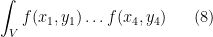
Now we consider the question of counting more general linear (or affine) patterns than arithmetic progressions. A reasonably general setting is to count patterns of the form

in a subset 


for some fixed integers 


where 

For instance, the task of counting arithmetic progressions 


where

Remark 1 One can replace the
norm on
in (9) with an
norm for various values of
. The set of all admissible
Improving this trivial bound turns out to be a key step in the theory of counting general linear patterns. In particular, it turns out that for any

except when 
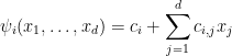
To reiterate: the key to the subject is to understand the inverse problem of characterising those functions 

This problem is of most interest (and the most difficult) in the “


Let us thus begin with analysing the 

and wish to classify the functions 


By the triangle inequality, we conclude that
On the other hand, we have the crude bound

Thus equality occurs, which (by the surjectivity hypothesis on all the 


and so from (10) one has the equation
for all 

So the problem now reduces to the algebraic problem of solving functional equations such as (11). To illustrate this type of problem, let us consider a simple case when 

in which case we are trying to understand solutions 

This equation involves three unknown functions 


applying 

thus 

for some constants 


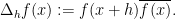
Returning now to the discrete world, we mimic the continuous operation of a partial derivative by introducing difference operators

for 


if we then difference in the 


for all 


Exercise 8 Let
be a function. Show that
if and only if one has
for some
and some homomorphism
. Conclude that the solutions to (12) are given by the form
, where
and
are homomorphisms with
.
Having solved the functional equation (12), let us now look at an equation related to four term arithmetic progressions, namely

for all 


In preparation for then eliminating

Differentiating in the

We shift

One final differentiation in 
For simplicity, we now make the assumption that the order 


for all 

Just as (affine-)linear functions can be completely described in terms of homomorphisms, quadratic functions can be described in terms of bilinear forms, as long as one avoids the characteristic
Exercise 9 Let
where
is a homomorphism, and
is a symmetric bihomomorphism (i.e.
, and
is a homomorphism in each of
individually (holding the other variable fixed)). (Hint: Heuristically, one should set
, but there is a difficulty because the operation of dividing by
is not well-defined on
roots of unity, thanks to

Exercise 10 Show that when
, that the complete solution to (13) is given by
for
,
, homomorphisms
, and symmetric bihomomorphisms
with
and
.

Exercise 11 Obtain a complete solution to the functional equation (13) in the case when
Exercise 12 Call a map
if one has
for all
. Show that if
obey the functional equation
and
, then
.

We are now ready to turn to the general case of solving equations of the form (11). We relied on two main tricks to solve these equations: differentiation, and change of variables. When solving an equation such as (13), we alternated these two tricks in turn. To handle the general case, it is more convenient to rearrange the argument by doing all the change of variables in advance. For instance, another way to solve (13) is to first make the (non-injective) change of variables

for arbitrary 

and (13) becomes

for all 


which soon places us back at (14) (assuming as before that
Now we can do the general case, once we put in place a definition (from this paper of mine with Ben Green):
Definition 1 (Cauchy-Schwarz complexity) A system
if, for every
, one can partition
into
classes (some of which may be empty), such that
) of the forms in any of these classes. The Cauchy-Schwarz complexity of a system is defined to be the least such
if no such
The adjective “Cauchy-Schwarz” (introduced by Gowers and Wolf) may be puzzling at present, but will be motivated later.
This is a somewhat strange definition to come to grips with at first, so we illustrate it with some examples. The system of forms 


Exercise 13 Show that for any
, the system of forms
has complexity
.
Exercise 14 Show that a system of non-constant forms has finite Cauchy-Schwarz complexity if and only if no form is an affine-linear combination of another.
There is an equivalent way to formulate the notion of Cauchy-Schwarz complexity, in the spirit of the change of variables mentioned earlier. Define the characteristic of a finite abelian group
Proposition 2 (Equivalent formulation of Cauchy-Schwarz complexity) Let
. Then
over
has non-zero
coefficients, but all the other forms
with
have at least one vanishing
is the linear form induced by the integer coefficients of
Proof: To show the “only if” part, observe that if 


then we obtain the claim.

Exercise 15 Let
. Suppose also that the characteristic of
are polynomials of degree
.
It turns out that this result is not quite best possible. Define the true complexity of a system of affine-linear forms 
Exercise 16 Show that the true complexity is always less than or equal to the Cauchy-Schwarz complexity, and give an example to show that strict inequality can occur. Also, show that the true complexity is finite if and only if the Cauchy-Schwarz complexity is finite.
Exercise 17 Show that Exercise 15 continues to hold if Cauchy-Schwarz complexity is replaced by true complexity. (Hint: first understand the cyclic case
, and use Exercise 15 to reduce to the case when all the
are polynomials of bounded degree. The main point is to use a “Lefschetz principle” to lift statements in
See this paper of Gowers and Wolf for further discussion of the relationship between Cauchy-Schwarz complexity and true complexity.
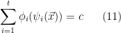
— 3. The Gowers uniformity norms —
In the previous section, we saw that equality in the trivial inequality (9) only occurred when the functions 

for all 

This phenomenon extends beyond the “

note that this is equivalent to (6). Using the identity

we easily verify that the expectation in the definition of (16) is a non-negative real. We also have the recursive formula

for all
The 

As such, it is actually a seminorm rather than a norm.
The 
Exercise 18 (Fourier representation of
of a finite abelian group
. For each function
by the formula
. Establish the identity

In particular, the 
For the higher Gowers norms, there is not nearly as nice a formula known in terms of things like the Fourier transform, and it is not immediately obvious that these are indeed norms. But this can be established by introducing the more general Gowers inner product
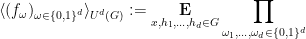

for any 


The relationship between the Gowers inner product and the Gowers uniformity norm is analogous to that between a Hilbert space inner product and the Hilbert space norm. In particular, we have the following analogue of the Cauchy-Schwarz inequality:
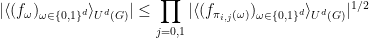
Exercise 19 (Cauchy-Schwarz-Gowers inequality) For any tuple
for all
, where for
and
,
is formed from
by replacing the
coordinate with
. Iterate this to conclude that
Then use this to conclude the monotonicity formula
for all
for all
. (Hint: For the latter inequality, raise both sides to the power
norms are indeed norms for all
.


The Gowers uniformity norms can be viewed as a quantitative measure of how well a given function behaves like a polynomial. One piece of evidence in this direction is:
Exercise 20 (Inverse conjecture for the Gowers norm,
, and let
. Show that
, with equality if and only if
for some polynomial
The problem of classifying smaller values of 
Exercise 21 (Polynomial phase invariance) If
. Conclude in particular that
where
ranges over polynomials of degree at most

The main utility for the Gowers norms in this subject comes from the fact that they control many other expressions of interest. Here is a basic example:
Exercise 22 Let
, let
be a function bounded in magnitude by
. Let
be non-zero integers, and suppose that the characteristic of
. Show that
Hint: induct on


This gives us an analogue of Exercise 15:
Exercise 23 (Generalised von Neumann inequality) Let
be a collection of affine-linear forms
with Cauchy-Schwarz complexity
whenever
are bounded in magnitude by one.
Conclude in particular that if
, then


From the above inequality, we see that if 

This is the initial motivation for studying inverse theorems for the Gowers norms, which give necessary conditions for a (bounded) function to have large 

30 comments
Comments feed for this article
27 April, 2010 at 11:24 am
mfrasca
Hi Terry,
There seem to be a lot of “Formula does not parse” messages. Is it just my problem?
Marco
28 April, 2010 at 2:29 pm
Joel Moreira
Dear Prof. Tao
In Exercise 3, I think something is missing, since q isn’t used (and the hint doesn’t seem to make sense)
28 April, 2010 at 2:43 pm
Terence Tao
Ah, there was a “mod q” missing in one of the displays. Thanks for the correction!
28 April, 2010 at 2:02 pm
jc
Not sure if this is the right place to post this, but I was browsing arxiv trackbacks and noticed that for your posts that link arxiv articles, in addition to the trackbacks expected, wordpress is also sending trackbacks for Thurston’s article linked in the sidebar.
See e.g. http://arxiv.org/tb/math/9404236
29 April, 2010 at 12:28 pm
Ryan
Does anyone else find that these 254B lecture notes posts do not show up in the RSS feed, or is it just me?
8 May, 2010 at 1:48 pm
254B, Lecture Notes 4: Equidistribution of polynomials over finite fields « What’s new
[…] from the previous notes that a function is a function is a polynomial of degree at most […]
19 May, 2010 at 11:38 pm
Pietro
Dear Terry,
in your definition of the Gowers inner product, I think you want to take the expectation over x,h_1,…,h_d of the expression that you have.
Thanks for the great notes and blog!
20 May, 2010 at 2:02 pm
Pietro
Also, in exercise 1, I guess we want the intersection of A and A+h to have size >> delta squared times N.
20 May, 2010 at 3:35 pm
Terence Tao
Thanks for the corrections!
20 May, 2010 at 9:44 pm
254B, Notes 5: The inverse conjecture for the Gowers norm I. The finite field case « What’s new
[…] regularity lemma, Gowers uniformity norms, polynomials, Szemeredi's theorem | by Terence Tao In Notes 3, we saw that the number of additive patterns in a given set was (in principle, at least) controlled […]
5 June, 2010 at 12:58 pm
254B, Lecture Notes 7: The transference principle, and linear equations in primes « What’s new
[…] will rely solely on the Cauchy-Schwarz inequality, using a weighted version of the arguments from Notes 3 that first appeared in this paper of Green and myself. We wish to control the […]
11 December, 2012 at 9:04 pm
Mixing for progressions in non-abelian groups « What’s new
[…] arguments let one conclude that are affine homomorphisms; see e.g. Section 2 of these lecture notes. It turns out that essentially the same argument can be applied in the nonabelian case, but one […]
30 March, 2013 at 4:27 am
Rex
Dear Terry,
There seems to be a discrepancy between the definition of the Gowers norm in “The primes contain arbitrarily long arithmetic progressions”:
versus the one used in the later “Linear equations” series:
Namely, the alternating conjugation is missing. Is there any particular reason for this change?
Of course, there is no difference when is real-valued, but “The primes contain…” remarks in the section on anti-uniformity that:
Given a polynomial of degree
  , we have
  , where
  . This comes from the fact that taking
  successive differences of
  gives the zero function.
For this example to work, it seems that we need the conjugation to be present.
30 March, 2013 at 7:48 am
Terence Tao
See Footnote 14 in the most recent version http://arxiv.org/abs/math/0404188 of the “The primes contain…” paper.
20 July, 2015 at 8:23 pm
A nonstandard analysis proof of Szemeredi’s theorem | What's new
[…] in numerous places in the literature (e.g. Lemma 11.4 of my book with Van Vu, or Exercise 23 of this blog post) and will not be repeated here. In particular, from multilinearity we see […]
14 August, 2018 at 6:12 am
farlabb
Dear professor Tao, , which has characteristic 3. For
  , take $a=2$ and the statement then is
  . But in this case one can just take a function which is nonzero on
  but 0 on the rest.
I am having struggles proving exercise 22. It seems as if I have found a counterexample. I looked at the group
I am also a little bit confused about your definition of affine linear form . You define it to be maps of the form
  for integers
  , but in a group, what does
  mean? If
  were a ring with unit, I would understand.
Thanks a lot in advance!
14 August, 2018 at 6:14 am
farlabb
Please ignore my first question (about counterexample as it is not correct what I wrote).
14 August, 2018 at 6:27 am
Terence Tao
Abelian groups are canonically modules over the integers, e.g., and
and  .
.
14 August, 2018 at 6:33 am
farlabb
Thanks for the reply. I understand it if you write where
where  and
and  , but how do I interpret
  as an element of
  ? Because in the definition of
  we write
  .
.
14 August, 2018 at 6:34 am
farlabb
Sorry for the typo, and
and  .
.
15 August, 2018 at 7:42 am
Terence Tao
This is a typo: should be an element of
  , not of
  . I will amend the text accordingly.
24 August, 2018 at 5:02 am
iPie
Hi prof. Tao, I find the proof of proposition 2 (equivalent formulation of CS-complexity) hard to follow (it could be me of course). I don’t understand how you use the large characteristic hypothesis to proof the “only if” part. Could you please explain it in more detail?
24 August, 2018 at 8:14 am
Terence Tao
Fix . By hypothesis, the rational form
  has non-vanishing
  coefficient. If the characteristic is large enough that it does not divide the numerator of this coefficient, this implies that the G-form
  also has non-vanishing coefficient. On the other hand, all the forms
  in the class associated to
  have vanishing
  coefficient. Hence
  cannot be an affine-linear combination of these
  .
.
7 June, 2020 at 6:06 am
Rok H.
Dear Professor Tao,
in the Exercise 8, it should be $a_1 = a_2 = – a_3$.
[Corrected, thanks – T.]
19 August, 2021 at 10:27 pm
Anonymous
I have a question about Exercise 5:
Set
 .
.
By equidistribution, it looks like
![|\{ (n,r) \in [N]^2 : (n,n-r,n-2r,n-3r) \in A \}| = ( N^2 + o_{N \to \infty}(1) ) \cdot \int_{y \cdot k_0= 0} \mathbf{1}_A(y) \ dy](https://s0.wp.com/latex.php?latex=%7C%5C%7B+%28n%2Cr%29+%5Cin+%5BN%5D%5E2+%3A+%28n%2Cn-r%2Cn-2r%2Cn-3r%29+%5Cin+A+%5C%7D%7C+%3D+%28+N%5E2+%2B+o_%7BN+%5Cto+%5Cinfty%7D%281%29+%29+%5Ccdot+%5Cint_%7By+%5Ccdot+k_0%3D+0%7D+%5Cmathbf%7B1%7D_A%28y%29+%5C+dy&bg=ffffff&fg=545454&s=0&c=20201002)
where
I’m getting a little confused because it looks to me like
 ,
,
which differs from the desired bound.
20 August, 2021 at 5:37 am
Terence Tao
The set you write is not well defined (if
  , then
  is not well-defined). You may be thinking of
  instead. In this case, the indicator function
  in your expression should be replaced by
 ![1_{[0,\delta]^4}](https://s0.wp.com/latex.php?latex=1_%7B%5B0%2C%5Cdelta%5D%5E4%7D&bg=ffffff&fg=545454&s=0&c=20201002) .
.
21 August, 2021 at 2:20 am
Anonymous
Thanks a lot!
13 November, 2021 at 3:49 am
Killua Zoldyck
Dear Prof. Tao, shouldn’t it be
  as the
  are taking values in
  .
.
In the statement below equation labelled
[Corrected, thanks – T.]
6 January, 2022 at 1:31 am
Killua Zoldyck
@Anonymous and @farlabb can we please connect via email at lucifer3099@gmail.com as i wanted to discuss some of the exercises.
28 January, 2022 at 6:09 am
Anonymous
Dear Prof Tao,
Can you please provide me with an hint on how to approach the exercise 4 in this section using the exercise 21 in section 1 (like explain how to work with the given hint) ? It is not very clear to me how to make use of exercise 21 in section 1.
[Approximate the cutoff![1_{[0,\delta]}( x \hbox{ mod } 1)](https://s0.wp.com/latex.php?latex=1_%7B%5B0%2C%5Cdelta%5D%7D%28+x+%5Chbox%7B+mod+%7D+1%29&bg=ffffff&fg=545454&s=0&c=20201002) by a trigonometric polynomial, so that the indicator function of
by a trigonometric polynomial, so that the indicator function of  can be approximated by a finite linear combination of functions of the forn
  . -T]
. -T]