You are currently browsing the yearly archive for 2011.

One of the most fundamental principles in Fourier analysis is the uncertainty principle. It does not have a single canonical formulation, but one typical informal description of the principle is that if a function {f} is restricted to a narrow region of physical space, then its Fourier transform {\hat f} must be necessarily “smeared out” over a broad region of frequency space. Some versions of the uncertainty principle are discussed in this previous blog post.

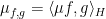
In this post I would like to highlight a useful instance of the uncertainty principle, due to Hugh Montgomery, which is useful in analytic number theory contexts. Specifically, suppose we are given a complex-valued function {f: {\bf Z} \rightarrow {\bf C}} on the integers. To avoid irrelevant issues at spatial infinity, we will assume that the support {\hbox{supp}(f) := \{ n \in {\bf Z}: f(n) \neq 0 \}} of this function is finite (in practice, we will only work with functions that are supported in an interval {[M+1,M+N]} for some natural numbers {M,N}). Then we can define the Fourier transform {\hat f: {\bf R}/{\bf Z} \rightarrow {\bf C}} by the formula

\displaystyle  \hat f(\xi) := \sum_{n \in {\bf Z}} f(n) e(-n\xi)

where {e(x) := e^{2\pi i x}}. (In some literature, the sign in the exponential phase is reversed, but this will make no substantial difference to the arguments below.)

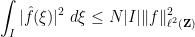
The classical uncertainty principle, in this context, asserts that if {f} is localised in an interval of length {N}, then {\hat f} must be “smeared out” at a scale of at least {1/N} (and essentially constant at scales less than {1/N}). For instance, if {f} is supported in {[M+1,M+N]}, then we have the Plancherel identity

\displaystyle  \int_{{\bf R}/{\bf Z}} |\hat f(\xi)|^2\ d\xi = \| f \|_{\ell^2({\bf Z})}^2 \ \ \ \ \ (1)

while from the Cauchy-Schwarz inequality we have

\displaystyle  |\hat f(\xi)| \leq N^{1/2} \| f \|_{\ell^2({\bf Z})}

for each frequency {\xi}, and in particular that

\displaystyle  \int_I |\hat f(\xi)|^2\ d\xi \leq N |I| \| f \|_{\ell^2({\bf Z})}^2

for any arc {I} in the unit circle (with {|I|} denoting the length of {I}). In particular, an interval of length significantly less than {1/N} can only capture a fraction of the {L^2} energy of the Fourier transform of {\hat f}, which is consistent with the above informal statement of the uncertainty principle.

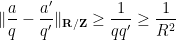
Another manifestation of the classical uncertainty principle is the large sieve inequality. A particularly nice formulation of this inequality is due independently to Montgomery and Vaughan and Selberg: if {f} is supported in {[M+1,M+N]}, and {\xi_1,\ldots,\xi_J} are frequencies in {{\bf R}/{\bf Z}} that are {\delta}-separated for some {\delta>0}, thus {\| \xi_i-\xi_j\|_{{\bf R}/{\bf Z}} \geq \delta} for all {1 \leq i<j \leq J} (where {\|\xi\|_{{\bf R}/{\bf Z}}} denotes the distance of {\xi} to the origin in {{\bf R}/{\bf Z}}), then

\displaystyle  \sum_{j=1}^J |\hat f(\xi_j)|^2 \leq (N + \frac{1}{\delta}) \| f \|_{\ell^2({\bf Z})}^2. \ \ \ \ \ (2)

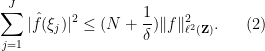
The reader is encouraged to see how this inequality is consistent with the Plancherel identity (1) and the intuition that {\hat f} is essentially constant at scales less than {1/N}. The factor {N + \frac{1}{\delta}} can in fact be amplified a little bit to {N + \frac{1}{\delta} - 1}, which is essentially optimal, by using a neat dilation trick of Paul Cohen, in which one dilates {[M+1,M+N]} to {[MK+K, MK+NK]} (and replaces each frequency {\xi_j} by their {K^{th}} roots), and then sending {K \rightarrow \infty} (cf. the tensor product trick); see this survey of Montgomery for details. But we will not need this refinement here.

In the above instances of the uncertainty principle, the concept of narrow support in physical space was formalised in the Archimedean sense, using the standard Archimedean metric {d_\infty(n,m) := |n-m|} on the integers {{\bf Z}} (in particular, the parameter {N} is essentially the Archimedean diameter of the support of {f}). However, in number theory, the Archimedean metric is not the only metric of importance on the integers; the {p}-adic metrics play an equally important role; indeed, it is common to unify the Archimedean and {p}-adic perspectives together into a unified adelic perspective. In the {p}-adic world, the metric balls are no longer intervals, but are instead residue classes modulo some power of {p}. Intersecting these balls from different {p}-adic metrics together, we obtain residue classes with respect to various moduli {q} (which may be either prime or composite). As such, another natural manifestation of the concept of “narrow support in physical space” is “vanishes on many residue classes modulo {q}“. This notion of narrowness is particularly common in sieve theory, when one deals with functions supported on thin sets such as the primes, which naturally tend to avoid many residue classes (particularly if one throws away the first few primes).

In this context, the uncertainty principle is this: the more residue classes modulo {q} that {f} avoids, the more the Fourier transform {\hat f} must spread out along multiples of {1/q}. To illustrate a very simple example of this principle, let us take {q=2}, and suppose that {f} is supported only on odd numbers (thus it completely avoids the residue class {0 \mod 2}). We write out the formulae for {\hat f(\xi)} and {\hat f(\xi+1/2)}:

\displaystyle  \hat f(\xi) = \sum_n f(n) e(-n\xi)

\displaystyle  \hat f(\xi+1/2) = \sum_n f(n) e(-n\xi) e(-n/2).

If {f} is supported on the odd numbers, then {e(-n/2)} is always equal to {-1} on the support of {f}, and so we have {\hat f(\xi+1/2)=-\hat f(\xi)}. Thus, whenever {\hat f} has a significant presence at a frequency {\xi}, it also must have an equally significant presence at the frequency {\xi+1/2}; there is a spreading out across multiples of {1/2}. Note that one has a similar effect if {f} was supported instead on the even integers instead of the odd integers.

A little more generally, suppose now that {f} avoids a single residue class modulo a prime {p}; for sake of argument let us say that it avoids the zero residue class {0 \mod p}, although the situation for the other residue classes is similar. For any frequency {\xi} and any {j=0,\ldots,p-1}, one has

\displaystyle  \hat f(\xi+j/p) = \sum_n f(n) e(-n\xi) e(-jn/p).

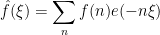
From basic Fourier analysis, we know that the phases {e(-jn/p)} sum to zero as {j} ranges from {0} to {p-1} whenever {n} is not a multiple of {p}. We thus have

\displaystyle  \sum_{j=0}^{p-1} \hat f(\xi+j/p) = 0.

In particular, if {\hat f(\xi)} is large, then one of the other {\hat f(\xi+j/p)} has to be somewhat large as well; using the Cauchy-Schwarz inequality, we can quantify this assertion in an {\ell^2} sense via the inequality

\displaystyle  \sum_{j=1}^{p-1} |\hat f(\xi+j/p)|^2 \geq \frac{1}{p-1} |\hat f(\xi)|^2. \ \ \ \ \ (3)

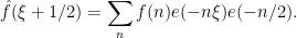
Let us continue this analysis a bit further. Now suppose that {f} avoids {\omega(p)} residue classes modulo a prime {p}, for some {0 \leq \omega(p) < p}. (We exclude the case {\omega(p)=p} as it is clearly degenerates by forcing {f} to be identically zero.) Let {\nu(n)} be the function that equals {1} on these residue classes and zero away from these residue classes, then

\displaystyle  \sum_n f(n) e(-n\xi) \nu(n) = 0.

Using the periodic Fourier transform, we can write

\displaystyle  \nu(n) = \sum_{j=0}^{p-1} c(j) e(-jn/p)

for some coefficients {c(j)}, thus

\displaystyle  \sum_{j=0}^{p-1} \hat f(\xi+j/p) c(j) = 0.

Some Fourier-analytic computations reveal that

\displaystyle  c(0) = \frac{\omega(p)}{p}

and

\displaystyle  \sum_{j=0}^{p-1} |c(j)|^2 = \frac{\omega(p)}{p}

and so after some routine algebra and the Cauchy-Schwarz inequality, we obtain a generalisation of (3):

\displaystyle  \sum_{j=1}^{p-1} |\hat f(\xi+j/p)|^2 \geq \frac{\omega(p)}{p-\omega(p)} |\hat f(\xi)|^2.

Thus we see that the more residue classes mod {p} we exclude, the more Fourier energy has to disperse along multiples of {1/p}. It is also instructive to consider the extreme case {\omega(p)=p-1}, in which {f} is supported on just a single residue class {a \mod p}; in this case, one clearly has {\hat f(\xi+j/p) = e(-aj/p) \hat f(\xi)}, and so {\hat f} spreads its energy completely evenly along multiples of {1/p}.

In 1968, Montgomery observed the following useful generalisation of the above calculation to arbitrary modulus:

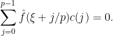
Proposition 1 (Montgomery’s uncertainty principle) Let {f: {\bf Z} \rightarrow{\bf C}} be a finitely supported function which, for each prime {p}, avoids {\omega(p)} residue classes modulo {p} for some {0 \leq \omega(p) < p}. Then for each natural number {q}, one has

\displaystyle  \sum_{1 \leq a \leq q: (a,q)=1} |\hat f(\xi+\frac{a}{q})|^2 \geq h(q) |\hat f(\xi)|^2

where {h(q)} is the quantity

\displaystyle  h(q) := \mu(q)^2 \prod_{p|q} \frac{\omega(p)}{p-\omega(p)} \ \ \ \ \ (4)

where {\mu} is the Möbius function.

We give a proof of this proposition below the fold.

Following the “adelic” philosophy, it is natural to combine this uncertainty principle with the large sieve inequality to take simultaneous advantage of localisation both in the Archimedean sense and in the {p}-adic senses. This leads to the following corollary:

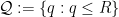
Corollary 2 (Arithmetic large sieve inequality) Let {f: {\bf Z} \rightarrow {\bf C}} be a function supported on an interval {[M+1,M+N]} which, for each prime {p}, avoids {\omega(p)} residue classes modulo {p} for some {0 \leq \omega(p) < p}. Let {\xi_1,\ldots,\xi_J \in {\bf R}/{\bf Z}}, and let {{\mathcal Q}} be a finite set of natural numbers. Suppose that the frequencies {\xi_j + \frac{a}{q}} with {1 \leq j \leq J}, {q \in {\mathcal Q}}, and {(a,q)=1} are {\delta}-separated. Then one has

\displaystyle  \sum_{j=1}^J |\hat f(\xi_j)|^2 \leq \frac{N + \frac{1}{\delta}}{\sum_{q \in {\mathcal Q}} h(q)} \| f \|_{\ell^2({\bf Z})}^2

where {h(q)} was defined in (4).

Indeed, from the large sieve inequality one has

\displaystyle  \sum_{j=1}^J \sum_{q \in {\mathcal Q}} \sum_{1 \leq a \leq q: (a,q)=1} |\hat f(\xi_j+\frac{a}{q})|^2 \leq (N + \frac{1}{\delta}) \| f \|_{\ell^2({\bf Z})}^2

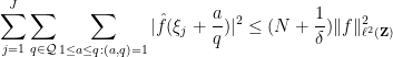
while from Proposition 1 one has

\displaystyle  \sum_{q \in {\mathcal Q}} \sum_{1 \leq a \leq q: (a,q)=1} |\hat f(\xi_j+\frac{a}{q})|^2 \geq (\sum_{q \in {\mathcal Q}} h(q)) |\hat f(\xi_j)|^2

whence the claim.

There is a great deal of flexibility in the above inequality, due to the ability to select the set {{\mathcal Q}}, the frequencies {\xi_1,\ldots,\xi_J}, the omitted classes {\omega(p)}, and the separation parameter {\delta}. Here is a typical application concerning the original motivation for the large sieve inequality, namely in bounding the size of sets which avoid many residue classes:

Corollary 3 (Large sieve) Let {A} be a set of integers contained in {[M+1,M+N]} which avoids {\omega(p)} residue classes modulo {p} for each prime {p}, and let {R>0}. Then

\displaystyle  |A| \leq \frac{N+R^2}{G(R)}

where

\displaystyle  G(R) := \sum_{q \leq R} h(q).

Proof: We apply Corollary 2 with {f = 1_A}, {J=1}, {\delta=1/R^2}, {\xi_1=0}, and {{\mathcal Q} := \{ q: q \leq R\}}. The key point is that the Farey sequence of fractions {a/q} with {q \leq R} and {(a,q)=1} is {1/R^2}-separated, since

\displaystyle  \| \frac{a}{q}-\frac{a'}{q'} \|_{{\bf R}/{\bf Z}} \geq \frac{1}{qq'} \geq \frac{1}{R^2}

whenever {a/q, a'/q'} are distinct fractions in this sequence. \Box

If, for instance, {A} is the set of all primes in {[M+1,M+N]} larger than {R}, then one can set {\omega(p)=1} for all {p \leq R}, which makes {h(q) = \frac{\mu^2(q)}{\phi(q)}}, where {\phi} is the Euler totient function. It is a classical estimate that

\displaystyle  G(R) = \log R + O(1).

Using this fact and optimising in {R}, we obtain (a special case of) the Brun-Titchmarsh inequality

\displaystyle  \pi(M+N)-\pi(M) \leq (2+o_{N \rightarrow \infty}(1)) \frac{N}{\log N}

where {\pi(x)} is the prime counting function; a variant of the same argument gives the more general Brun-Titchmarsh inequality

\displaystyle  \pi(M+N;a,q)-\pi(M;a,q) \leq (2+o_{N \rightarrow \infty;q}(1)) \frac{q}{\phi(q)} \frac{N}{\log N}

for any primitive residue class {a \mod q}, where {\pi(M;a,q)} is the number of primes less than or equal to {M} that are congruent to {a \mod q}. By performing a more careful optimisation using a slightly sharper version of the large sieve inequality (2) that exploits the irregular spacing of the Farey sequence, Montgomery and Vaughan were able to delete the error term in the Brun-Titchmarsh inequality, thus establishing the very nice inequality

\displaystyle  \pi(M+N;a,q)-\pi(M;a,q) \leq 2 \frac{q}{\phi(q)} \frac{N}{\log N}

for any natural numbers {M,N,a,q} with {N>1}. This is a particularly useful inequality in non-asymptotic analytic number theory (when one wishes to study number theory at explicit orders of magnitude, rather than the number theory of sufficiently large numbers), due to the absence of asymptotic notation.

I recently realised that Corollary 2 also establishes a stronger version of the “restriction theorem for the Selberg sieve” that Ben Green and I proved some years ago (indeed, one can view Corollary 2 as a “restriction theorem for the large sieve”). I’m placing the details below the fold.

Read the rest of this entry »

In 1964, Kemperman established the following result:

Theorem 1 Let {G} be a compact connected group, with a Haar probability measure {\mu}. Let {A, B} be compact subsets of {G}. Then

\displaystyle \mu(AB) \geq \min( \mu(A) + \mu(B), 1 ).

Remark 1 The estimate is sharp, as can be seen by considering the case when {G} is a unit circle, and {A, B} are arcs; similarly if {G} is any compact connected group that projects onto the circle. The connectedness hypothesis is essential, as can be seen by considering what happens if {A} and {B} are a non-trivial open subgroup of {G}. For locally compact connected groups which are unimodular but not compact, there is an analogous statement, but with {\mu} now a Haar measure instead of a Haar probability measure, and the right-hand side {\min(\mu(A)+\mu(B),1)} replaced simply by {\mu(A)+\mu(B)}. The case when {G} is a torus is due to Macbeath, and the case when {G} is a circle is due to Raikov. The theorem is closely related to the Cauchy-Davenport inequality; indeed, it is not difficult to use that inequality to establish the circle case, and the circle case can be used to deduce the torus case by considering increasingly dense circle subgroups of the torus (alternatively, one can also use Kneser’s theorem).

By inner regularity, the hypothesis that {A,B} are compact can be replaced with Borel measurability, so long as one then adds the additional hypothesis that {A+B} is also Borel measurable.

A short proof of Kemperman’s theorem was given by Ruzsa. In this post I wanted to record how this argument can be used to establish the following more “robust” version of Kemperman’s theorem, which not only lower bounds {AB}, but gives many elements of {AB} some multiplicity:

Theorem 2 Let {G} be a compact connected group, with a Haar probability measure {\mu}. Let {A, B} be compact subsets of {G}. Then for any {0 \leq t \leq \min(\mu(A),\mu(B))}, one has

\displaystyle \int_G \min(1_A*1_B, t)\ d\mu \geq t \min(\mu(A)+\mu(B) - t,1). \ \ \ \ \ (1)


Indeed, Theorem 1 can be deduced from Theorem 2 by dividing (1) by {t} and then taking limits as {t \rightarrow 0}. The bound in (1) is sharp, as can again be seen by considering the case when {A,B} are arcs in a circle. The analogous claim for cyclic groups for prime order was established by Pollard, and for general abelian groups by Green and Ruzsa.

Let us now prove Theorem 2. It uses a submodularity argument related to one discussed in this previous post. We fix {B} and {t} with {0 \leq t \leq \mu(B)}, and define the quantity

\displaystyle c(A) := \int_G \min(1_A*1_B, t)\ d\mu - t (\mu(A)+\mu(B)-t).

for any compact set {A}. Our task is to establish that {c(A) \geq 0} whenever {t \leq \mu(A) \leq 1-\mu(B)+t}.

We first verify the extreme cases. If {\mu(A) = t}, then {1_A*1_B \leq t}, and so {c(A)=0} in this case (since {\int_G 1_A*1_B = \mu(A)\mu(B) = t \mu(B)}). At the other extreme, if {\mu(A) = 1-\mu(B)+t}, then from the inclusion-exclusion principle we see that {1_A * 1_B \geq t}, and so again {c(A)=0} in this case.

To handle the intermediate regime when {\mu(A)} lies between {t} and {1-\mu(B)+t}, we rely on the submodularity inequality

\displaystyle c(A_1) + c(A_2) \geq c(A_1 \cap A_2) + c(A_1 \cup A_2) \ \ \ \ \ (2)


for arbitrary compact {A_1,A_2}. This inequality comes from the obvious pointwise identity

\displaystyle 1_{A_1} + 1_{A_2} = 1_{A_1 \cap A_2} + 1_{A_1 \cup A_2}

whence

\displaystyle 1_{A_1}*1_B + 1_{A_2}*1_B = 1_{A_1 \cap A_2}*1_B + 1_{A_1 \cup A_2}*1_B

and thus (noting that the quantities on the left are closer to each other than the quantities on the right)

\displaystyle \min(1_{A_1}*1_B,t) + \min(1_{A_2}*1_B,t)

\displaystyle \geq \min(1_{A_1 \cap A_2}*1_B,t) + \min(1_{A_1 \cup A_2}*1_B,t)

at which point (2) follows by integrating over {G} and then using the inclusion-exclusion principle.

Now introduce the function

\displaystyle f(a) := \inf \{ c(A) : \mu(A) = a \}

for {t \leq a \leq 1-\mu(B)+t}. From the preceding discussion {f(a)} vanishes at the endpoints {a = t, 1-\mu(B)+t}; our task is to show that {f(a)} is non-negative in the interior region {t < a < 1-\mu(B)+t}. Suppose for contradiction that this was not the case. It is easy to see that {f} is continuous (indeed, it is even Lipschitz continuous), so there must be {t < a < 1-\mu(B)+t} at which {f} is a local minimum and not locally constant. In particular, {0 <a <1}. But for any {A} with {\mu(A) = a}, we have the translation-invariance

\displaystyle c(gA) = c(A) \ \ \ \ \ (3)


for any {g \in G}, and hence by (2)

\displaystyle c(A) \geq \frac{1}{2} c(A \cap gA) + \frac{1}{2} c(A \cup gA ).

Note that {\mu(A \cap gA)} depends continuously on {g}, equals {a} when {g} is the identity, and has an average value of {a^2}. As {G} is connected, we thus see from the intermediate value theorem that for any {0 < \epsilon < a-a^2}, we can find {g} such that {\mu(A \cap gA) = a-\epsilon}, and thus by inclusion-exclusion {\mu(A \cup gA) = a+\epsilon}. By definition of {f}, we thus have

\displaystyle c(A) \geq \frac{1}{2} f(a-\epsilon) + \frac{1}{2} f(a+\epsilon).

Taking infima in {A} (and noting that the hypotheses on {\epsilon} are independent of {A}) we conclude that

\displaystyle f(a) \geq \frac{1}{2} f(a-\epsilon) + \frac{1}{2} f(a+\epsilon)

for all {0 < \epsilon < a-a^2}. As {f} is a local minimum and {\epsilon} is arbitrarily small, this implies that {f} is locally constant, a contradiction. This establishes Theorem 2.

We observe the following corollary:

Corollary 3 Let {G} be a compact connected group, with a Haar probability measure {\mu}. Let {A, B, C} be compact subsets of {G}, and let {\delta := \min(\mu(A),\mu(B),\mu(C))}. Then one has the pointwise estimate

\displaystyle 1_A * 1_B * 1_C \geq \frac{1}{4} (\mu(A)+\mu(B)+\mu(C)-1)_+^2

if {\mu(A)+\mu(B)+\mu(C)-1 \leq 2 \delta}, and

\displaystyle 1_A * 1_B * 1_C \geq \delta (\mu(A)+\mu(B)+\mu(C)-1-\delta)

if {\mu(A)+\mu(B)+\mu(C)-1 \geq 2 \delta}.

Once again, the bounds are completely sharp, as can be seen by computing {1_A*1_B*1_C} when {A,B,C} are arcs of a circle. For quasirandom {G}, one can do much better than these bounds, as discussed in this recent blog post; thus, the abelian case is morally the worst case here, although it seems difficult to convert this intuition into a rigorous reduction.

Proof: By cyclic permutation we may take {\delta = \mu(C)}. For any

\displaystyle (\mu(A)+\mu(B)-1)_+ \leq t \leq \min(\mu(A),\mu(B)),

we can bound

\displaystyle 1_A*1_B*1_C \geq \min(1_A*1_B,t)*1_C

\displaystyle \geq \int_G \min(1_A*1_B,t)\ d\mu - t (1-\mu(C))

\displaystyle \geq t (\mu(A)+\mu(B)-t) - t (1-\mu(C))

\displaystyle = t \min( \mu(A)+\mu(B)+\mu(C)-1-t )

where we used Theorem 2 to obtain the third line. Optimising in {t}, we obtain the claim. \Box

Emmanuel Breuillard, Ben Green and I have just uploaded to the arXiv the short paper “A nilpotent Freiman dimension lemma“, submitted to the special volume of the European Journal of Combinatorics in honour of Yahya Ould Hamidoune.  This paper is a nonabelian (or more precisely, nilpotent) variant of the following additive combinatorics lemma of Freiman:

Freiman’s lemma.  Let A be a finite subset of a Euclidean space with |A+A| \leq K|A|.  Then A is contained in an affine subspace of dimension at most {}\lfloor K-1 \rfloor.

This can be viewed as a “cheap” version of the more well known theorem of Freiman that places sets of small doubling in a torsion-free abelian group inside a generalised arithmetic progression.  The advantage here is that the bound on the dimension is extremely explicit.

Our main result is

Theorem.  Let A be a finite subset of a simply-connected nilpotent Lie group G which is a K-approximate group (i.e. A is symmetric, contains the identity, and A \cdot A can be covered by up to K left translates of A.  Then A can be covered by at most K^{2+29K^9} left-translates of a closed connected Lie subgroup of dimension at most K^9.

We remark that our previous paper established a similar result, in which the dimension bound was improved to 6\log_2 K, but at the cost of worsening the covering number to O_K(1), and with a much more complicated proof  (91 pages instead of 8). Furthermore, the bound on O_K(1) is ineffective, due to the use of ultraproducts in the argument (though it is likely that some extremely lousy explicit bound could eventually be squeezed out of the argument by finitising everything).  Note that the step of the ambient nilpotent group G does not influence the final bounds in the theorem, although we do of course need this step to be finite.  A simple quotienting argument allows one to deduce a corollary of the above theorem in which the ambient group is assumed to be residually torsion-free nilpotent instead of being a simply connected nilpotent Lie group, but we omit the statement of this corollary here.

To motivate the proof of this theorem, let us first show a simple case of an argument of Gleason, which is very much in the spirit of Freiman’s lemma:

Gleason Lemma (special case).  Let A be a finite symmetric subset of a Euclidean space, and let 0 = H_0 \subset H_1 \subset \ldots \subset H_k be a sequence of subspaces in this space, such that the sets 2A \cap H_i are strictly increasing in i for i=0,\ldots,k.  Then |5A| \geq k|A|, where 5A = A+A+A+A+A.

Proof.    By hypothesis, for each i=1,\ldots,k, the projection B_i of 2A \cap H_i to H_i / H_{i-1} is non-trivial, finite, and symmetric.   In particular, since the vector space H_i/H_{i-1} is torsion-free, B_i+B_i is strictly larger than B_i.  Equivalently, one can find a_i in (2A \cap H_i) + (2A \cap H_i) that does not lie in (2A \cap H_i) + H_{i-1}; in particular, a_i \in 4A \cap H_i and a_i+A is disjoint from H_{i-1}+A.  As a consequence, the a_i+A are disjoint and lie in 5A, whence the claim. \Box

Note that by combining the contrapositive of this lemma with a greedy algorithm, one can show that any K-approximate group in a Euclidean space is contained in a subspace of dimension at most K^4, which is a weak version of Freiman’s lemma.

To extend the argument to the nilpotent setting we use the following idea.  Observe that any non-trivial genuine subgroup H of a nilpotent group G will contain at least one non-trivial central element; indeed, by intersecting H with the lower central series G = G_1 \geq G_2 \geq G_3 \geq \ldots of G, and considering the last intersection H \cap G_k which is non-trivial, one obtains the claim.  It turns out that one can adapt this argument to approximate groups, so that any sufficiently large K-approximate subgroup A of G will contain a non-trivial element that centralises a large fraction of A.  Passing to this large fraction and quotienting out the central element, we obtain a new approximate group.    If, after a bounded number of steps, this procedure gives an approximate group of bounded size, we are basically done.  If, however, the process continues, then by using some Lie group theory, one can find a long sequence H_0 \leq H_1 \leq \ldots \leq H_k of connected Lie subgroups of G, such that the sets A^2 \cap H_i are strictly increasing in i.   Using some Lie group theory and the hypotheses on G, one can deduce that the group \langle A^2 \cap H_{i+1}\rangle generated by A^2 \cap H_{i+1} is much larger than \langle A^2 \cap H_i \rangle, in the sense that the latter group has infinite index in the former.   It then turns out that the Gleason argument mentioned above can be adapted to this setting.

LLet {L: H \rightarrow H} be a self-adjoint operator on a finite-dimensional Hilbert space {H}. The behaviour of this operator can be completely described by the spectral theorem for finite-dimensional self-adjoint operators (i.e. Hermitian matrices, when viewed in coordinates), which provides a sequence {\lambda_1,\ldots,\lambda_n \in {\bf R}} of eigenvalues and an orthonormal basis {e_1,\ldots,e_n} of eigenfunctions such that {L e_i = \lambda_i e_i} for all {i=1,\ldots,n}. In particular, given any function {m: \sigma(L) \rightarrow {\bf C}} on the spectrum {\sigma(L) := \{ \lambda_1,\ldots,\lambda_n\}} of {L}, one can then define the linear operator {m(L): H \rightarrow H} by the formula

\displaystyle m(L) e_i := m(\lambda_i) e_i,

which then gives a functional calculus, in the sense that the map {m \mapsto m(L)} is a {C^*}-algebra isometric homomorphism from the algebra {BC(\sigma(L) \rightarrow {\bf C})} of bounded continuous functions from {\sigma(L)} to {{\bf C}}, to the algebra {B(H \rightarrow H)} of bounded linear operators on {H}. Thus, for instance, one can define heat operators {e^{-tL}} for {t>0}, Schrödinger operators {e^{itL}} for {t \in {\bf R}}, resolvents {\frac{1}{L-z}} for {z \not \in \sigma(L)}, and (if {L} is positive) wave operators {e^{it\sqrt{L}}} for {t \in {\bf R}}. These will be bounded operators (and, in the case of the Schrödinger and wave operators, unitary operators, and in the case of the heat operators with {L} positive, they will be contractions). Among other things, this functional calculus can then be used to solve differential equations such as the heat equation

\displaystyle u_t + Lu = 0; \quad u(0) = f \ \ \ \ \ (1)


the Schrödinger equation

\displaystyle u_t + iLu = 0; \quad u(0) = f \ \ \ \ \ (2)


the wave equation

\displaystyle u_{tt} + Lu = 0; \quad u(0) = f; \quad u_t(0) = g \ \ \ \ \ (3)


or the Helmholtz equation

\displaystyle (L-z) u = f. \ \ \ \ \ (4)


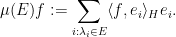
The functional calculus can also be associated to a spectral measure. Indeed, for any vectors {f, g \in H}, there is a complex measure {\mu_{f,g}} on {\sigma(L)} with the property that

\displaystyle \langle m(L) f, g \rangle_H = \int_{\sigma(L)} m(x) d\mu_{f,g}(x);

indeed, one can set {\mu_{f,g}} to be the discrete measure on {\sigma(L)} defined by the formula

\displaystyle \mu_{f,g}(E) := \sum_{i: \lambda_i \in E} \langle f, e_i \rangle_H \langle e_i, g \rangle_H.

One can also view this complex measure as a coefficient

\displaystyle \mu_{f,g} = \langle \mu f, g \rangle_H

of a projection-valued measure {\mu} on {\sigma(L)}, defined by setting

\displaystyle \mu(E) f := \sum_{i: \lambda_i \in E} \langle f, e_i \rangle_H e_i.

Finally, one can view {L} as unitarily equivalent to a multiplication operator {M: f \mapsto g f} on {\ell^2(\{1,\ldots,n\})}, where {g} is the real-valued function {g(i) := \lambda_i}, and the intertwining map {U: \ell^2(\{1,\ldots,n\}) \rightarrow H} is given by

\displaystyle U ( (c_i)_{i=1}^n ) := \sum_{i=1}^n c_i e_i,

so that {L = U M U^{-1}}.

It is an important fact in analysis that many of these above assertions extend to operators on an infinite-dimensional Hilbert space {H}, so long as one one is careful about what “self-adjoint operator” means; these facts are collectively referred to as the spectral theorem. For instance, it turns out that most of the above claims have analogues for bounded self-adjoint operators {L: H \rightarrow H}. However, in the theory of partial differential equations, one often needs to apply the spectral theorem to unbounded, densely defined linear operators {L: D \rightarrow H}, which (initially, at least), are only defined on a dense subspace {D} of the Hilbert space {H}. A very typical situation arises when {H = L^2(\Omega)} is the square-integrable functions on some domain or manifold {\Omega} (which may have a boundary or be otherwise “incomplete”), and {D = C^\infty_c(\Omega)} are the smooth compactly supported functions on {\Omega}, and {L} is some linear differential operator. It is then of interest to obtain the spectral theorem for such operators, so that one build operators such as {e^{-tL}, e^{itL}, \frac{1}{L-z}, e^{it\sqrt{L}}} or to solve equations such as (1), (2), (3), (4).

In order to do this, some necessary conditions on the densely defined operator {L: D \rightarrow H} must be imposed. The most obvious is that of symmetry, which asserts that

\displaystyle \langle Lf, g \rangle_H = \langle f, Lg \rangle_H \ \ \ \ \ (5)


for all {f, g \in D}. In some applications, one also wants to impose positive definiteness, which asserts that

\displaystyle \langle Lf, f \rangle_H \geq 0 \ \ \ \ \ (6)


for all {f \in D}. These hypotheses are sufficient in the case when {L} is bounded, and in particular when {H} is finite dimensional. However, as it turns out, for unbounded operators these conditions are not, by themselves, enough to obtain a good spectral theory. For instance, one consequence of the spectral theorem should be that the resolvents {(L-z)^{-1}} are well-defined for any strictly complex {z}, which by duality implies that the image of {L-z} should be dense in {H}. However, this can fail if one just assumes symmetry, or symmetry and positive definiteness. A well-known example occurs when {H} is the Hilbert space {H := L^2((0,1))}, {D := C^\infty_c((0,1))} is the space of test functions, and {L} is the one-dimensional Laplacian {L := -\frac{d^2}{dx^2}}. Then {L} is symmetric and positive, but the operator {L-k^2} does not have dense image for any complex {k}, since

\displaystyle \langle (L-\overline{k}^2) f, e^{\overline{k}x} \rangle_H = 0

for all test functions {f \in C^\infty_c((0,1))}, as can be seen from a routine integration by parts. As such, the resolvent map is not everywhere uniquely defined. There is also a lack of uniqueness for the wave, heat, and Schrödinger equations for this operator (note that there are no spatial boundary conditions specified in these equations).

Another example occurs when {H := L^2((0,+\infty))}, {D := C^\infty_c((0,+\infty))}, {L} is the momentum operator {L := i \frac{d}{dx}}. Then the resolvent {(L-z)^{-1}} can be uniquely defined for {z} in the upper half-plane, but not in the lower half-plane, due to the obstruction

\displaystyle \langle (L-z) f, e^{i \bar{z} x} \rangle_H = 0

for all test functions {f} (note that the function {e^{i\bar{z} x}} lies in {L^2((0,+\infty))} when {z} is in the lower half-plane). For related reasons, the translation operators {e^{itL}} have a problem with either uniqueness or existence (depending on whether {t} is positive or negative), due to the unspecified boundary behaviour at the origin.

The key property that lets one avoid this bad behaviour is that of essential self-adjointness. Once {L} is essentially self-adjoint, then spectral theorem becomes applicable again, leading to all the expected behaviour (e.g. existence and uniqueness for the various PDE given above).

Unfortunately, the concept of essential self-adjointness is defined rather abstractly, and is difficult to verify directly; unlike the symmetry condition (5) or the positive condition (6), it is not a “local” condition that can be easily verified just by testing {L} on various inputs, but is instead a more “global” condition. In practice, to verify this property, one needs to invoke one of a number of a partial converses to the spectral theorem, which roughly speaking asserts that if at least one of the expected consequences of the spectral theorem is true for some symmetric densely defined operator {L}, then {L} is self-adjoint. Examples of “expected consequences” include:

  • Existence of resolvents {(L-z)^{-1}} (or equivalently, dense image for {L-z});
  • Existence of a contractive heat propagator semigroup {e^{tL}} (in the positive case);
  • Existence of a unitary Schrödinger propagator group {e^{itL}};
  • Existence of a unitary wave propagator group {e^{it\sqrt{L}}} (in the positive case);
  • Existence of a “reasonable” functional calculus.
  • Unitary equivalence with a multiplication operator.

Thus, to actually verify essential self-adjointness of a differential operator, one typically has to first solve a PDE (such as the wave, Schrödinger, heat, or Helmholtz equation) by some non-spectral method (e.g. by a contraction mapping argument, or a perturbation argument based on an operator already known to be essentially self-adjoint). Once one can solve one of the PDEs, then one can apply one of the known converse spectral theorems to obtain essential self-adjointness, and then by the forward spectral theorem one can then solve all the other PDEs as well. But there is no getting out of that first step, which requires some input (typically of an ODE, PDE, or geometric nature) that is external to what abstract spectral theory can provide. For instance, if one wants to establish essential self-adjointness of the Laplace-Beltrami operator {L = -\Delta_g} on a smooth Riemannian manifold {(M,g)} (using {C^\infty_c(M)} as the domain space), it turns out (under reasonable regularity hypotheses) that essential self-adjointness is equivalent to geodesic completeness of the manifold, which is a global ODE condition rather than a local one: one needs geodesics to continue indefinitely in order to be able to (unitarily) solve PDEs such as the wave equation, which in turn leads to essential self-adjointness. (Note that the domains {(0,1)} and {(0,+\infty)} in the previous examples were not geodesically complete.) For this reason, essential self-adjointness of a differential operator is sometimes referred to as quantum completeness (with the completeness of the associated Hamilton-Jacobi flow then being the analogous classical completeness).

In these notes, I wanted to record (mostly for my own benefit) the forward and converse spectral theorems, and to verify essential self-adjointness of the Laplace-Beltrami operator on geodesically complete manifolds. This is extremely standard analysis (covered, for instance, in the texts of Reed and Simon), but I wanted to write it down myself to make sure that I really understood this foundational material properly.

Read the rest of this entry »

In the previous set of notes we saw how a representation-theoretic property of groups, namely Kazhdan’s property (T), could be used to demonstrate expansion in Cayley graphs. In this set of notes we discuss a different representation-theoretic property of groups, namely quasirandomness, which is also useful for demonstrating expansion in Cayley graphs, though in a somewhat different way to property (T). For instance, whereas property (T), being qualitative in nature, is only interesting for infinite groups such as {SL_d({\bf Z})} or {SL_d({\bf R})}, and only creates Cayley graphs after passing to a finite quotient, quasirandomness is a quantitative property which is directly applicable to finite groups, and is able to deduce expansion in a Cayley graph, provided that random walks in that graph are known to become sufficiently “flat” in a certain sense.

The definition of quasirandomness is easy enough to state:

Definition 1 (Quasirandom groups) Let {G} be a finite group, and let {D \geq 1}. We say that {G} is {D}-quasirandom if all non-trivial unitary representations {\rho: G \rightarrow U(H)} of {G} have dimension at least {D}. (Recall a representation is trivial if {\rho(g)} is the identity for all {g \in G}.)

Exercise 1 Let {G} be a finite group, and let {D \geq 1}. A unitary representation {\rho: G \rightarrow U(H)} is said to be irreducible if {H} has no {G}-invariant subspaces other than {\{0\}} and {H}. Show that {G} is {D}-quasirandom if and only if every non-trivial irreducible representation of {G} has dimension at least {D}.

Remark 1 The terminology “quasirandom group” was introduced explicitly (though with slightly different notational conventions) by Gowers in 2008 in his detailed study of the concept; the name arises because dense Cayley graphs in quasirandom groups are quasirandom graphs in the sense of Chung, Graham, and Wilson, as we shall see below. This property had already been used implicitly to construct expander graphs by Sarnak and Xue in 1991, and more recently by Gamburd in 2002 and by Bourgain and Gamburd in 2008. One can of course define quasirandomness for more general locally compact groups than the finite ones, but we will only need this concept in the finite case. (A paper of Kunze and Stein from 1960, for instance, exploits the quasirandomness properties of the locally compact group {SL_2({\bf R})} to obtain mixing estimates in that group.)

Quasirandomness behaves fairly well with respect to quotients and short exact sequences:

Exercise 2 Let {0 \rightarrow H \rightarrow G \rightarrow K \rightarrow 0} be a short exact sequence of finite groups {H,G,K}.

  • (i) If {G} is {D}-quasirandom, show that {K} is {D}-quasirandom also. (Equivalently: any quotient of a {D}-quasirandom finite group is again a {D}-quasirandom finite group.)
  • (ii) Conversely, if {H} and {K} are both {D}-quasirandom, show that {G} is {D}-quasirandom also. (In particular, the direct or semidirect product of two {D}-quasirandom finite groups is again a {D}-quasirandom finite group.)

Informally, we will call {G} quasirandom if it is {D}-quasirandom for some “large” {D}, though the precise meaning of “large” will depend on context. For applications to expansion in Cayley graphs, “large” will mean “{D \geq |G|^c} for some constant {c>0} independent of the size of {G}“, but other regimes of {D} are certainly of interest.

The way we have set things up, the trivial group {G = \{1\}} is infinitely quasirandom (i.e. it is {D}-quasirandom for every {D}). This is however a degenerate case and will not be discussed further here. In the non-trivial case, a finite group can only be quasirandom if it is large and has no large subgroups:

Exercise 3 Let {D \geq 1}, and let {G} be a finite {D}-quasirandom group.

  • (i) Show that if {G} is non-trivial, then {|G| \geq D+1}. (Hint: use the mean zero component {\tau\downharpoonright_{\ell^2(G)_0}} of the regular representation {\tau: G \rightarrow U(\ell^2(G))}.) In particular, non-trivial finite groups cannot be infinitely quasirandom.
  • (ii) Show that any proper subgroup {H} of {G} has index {[G:H] \geq D+1}. (Hint: use the mean zero component of the quasiregular representation.)

The following exercise shows that quasirandom groups have to be quite non-abelian, and in particular perfect:

Exercise 4 (Quasirandomness, abelianness, and perfection) Let {G} be a finite group.

  • (i) If {G} is abelian and non-trivial, show that {G} is not {2}-quasirandom. (Hint: use Fourier analysis or the classification of finite abelian groups.)
  • (ii) Show that {G} is {2}-quasirandom if and only if it is perfect, i.e. the commutator group {[G,G]} is equal to {G}. (Equivalently, {G} is {2}-quasirandom if and only if it has no non-trivial abelian quotients.)

Later on we shall see that there is a converse to the above two exercises; any non-trivial perfect finite group with no large subgroups will be quasirandom.

Exercise 5 Let {G} be a finite {D}-quasirandom group. Show that for any subgroup {G'} of {G}, {G'} is {D/[G:G']}-quasirandom, where {[G:G'] := |G|/|G'|} is the index of {G'} in {G}. (Hint: use induced representations.)

Now we give an example of a more quasirandom group.

Lemma 2 (Frobenius lemma) If {F_p} is a field of some prime order {p}, then {SL_2(F_p)} is {\frac{p-1}{2}}-quasirandom.

This should be compared with the cardinality {|SL_2(F_p)|} of the special linear group, which is easily computed to be {(p^2-1) \times p = p^3 - p}.

Proof: We may of course take {p} to be odd. Suppose for contradiction that we have a non-trivial representation {\rho: SL_2(F_p) \rightarrow U_d({\bf C})} on a unitary group of some dimension {d} with {d < \frac{p-1}{2}}. Set {a} to be the group element

\displaystyle a := \begin{pmatrix} 1 & 1 \\ 0 & 1 \end{pmatrix},

and suppose first that {\rho(a)} is non-trivial. Since {a^p=1}, we have {\rho(a)^p=1}; thus all the eigenvalues of {\rho(a)} are {p^{th}} roots of unity. On the other hand, by conjugating {a} by diagonal matrices in {SL_2(F_p)}, we see that {a} is conjugate to {a^m} (and hence {\rho(a)} conjugate to {\rho(a)^m}) whenever {m} is a quadratic residue mod {p}. As such, the eigenvalues of {\rho(a)} must be permuted by the operation {x \mapsto x^m} for any quadratic residue mod {p}. Since {\rho(a)} has at least one non-trivial eigenvalue, and there are {\frac{p-1}{2}} distinct quadratic residues, we conclude that {\rho(a)} has at least {\frac{p-1}{2}} distinct eigenvalues. But {\rho(a)} is a {d \times d} matrix with {d < \frac{p-1}{2}}, a contradiction. Thus {a} lies in the kernel of {\rho}. By conjugation, we then see that this kernel contains all unipotent matrices. But these matrices generate {SL_2(F_p)} (see exercise below), and so {\rho} is trivial, a contradiction. \Box

Exercise 6 Show that for any prime {p}, the unipotent matrices

\displaystyle \begin{pmatrix} 1 & t \\ 0 & 1 \end{pmatrix}, \begin{pmatrix} 1 & 0 \\ t & 1 \end{pmatrix}

for {t} ranging over {F_p} generate {SL_2(F_p)} as a group.

Exercise 7 Let {G} be a finite group, and let {D \geq 1}. If {G} is generated by a collection {G_1,\ldots,G_k} of {D}-quasirandom subgroups, show that {G} is itself {D}-quasirandom.

Exercise 8 Show that {SL_d(F_p)} is {\frac{p-1}{2}}-quasirandom for any {d \geq 2} and any prime {p}. (This is not sharp; the optimal bound here is {\gg_d p^{d-1}}, which follows from the results of Landazuri and Seitz.)

As a corollary of the above results and Exercise 2, we see that the projective special linear group {PSL_d(F_p)} is also {\frac{p-1}{2}}-quasirandom.

Remark 2 One can ask whether the bound {\frac{p-1}{2}} in Lemma 2 is sharp, assuming of course that {p} is odd. Noting that {SL_2(F_p)} acts linearly on the plane {F_p^2}, we see that it also acts projectively on the projective line {PF_p^1 := (F_p^2 \backslash \{0\}) / F_p^\times}, which has {p+1} elements. Thus {SL_2(F_p)} acts via the quasiregular representation on the {p+1}-dimensional space {\ell^2(PF_p^1)}, and also on the {p}-dimensional subspace {\ell^2(PF_p^1)_0}; this latter representation (known as the Steinberg representation) is irreducible. This shows that the {\frac{p-1}{2}} bound cannot be improved beyond {p}. More generally, given any character {\chi: F_p^\times \rightarrow S^1}, {SL_2(F_p)} acts on the {p+1}-dimensional space {V_\chi} of functions {f \in \ell^2( F_p^2 \backslash \{0\} )} that obey the twisted dilation invariance {f(tx) = \chi(t) f(x)} for all {t \in F_p^\times} and {x \in F_p^2 \backslash \{0\}}; these are known as the principal series representations. When {\chi} is the trivial character, this is the quasiregular representation discussed earlier. For most other characters, this is an irreducible representation, but it turns out that when {\chi} is the quadratic representation (thus taking values in {\{-1,+1\}} while being non-trivial), the principal series representation splits into the direct sum of two {\frac{p+1}{2}}-dimensional representations, which comes very close to matching the bound in Lemma 2. There is a parallel series of representations to the principal series (known as the discrete series) which is more complicated to describe (roughly speaking, one has to embed {F_p} in a quadratic extension {F_{p^2}} and then use a rotated version of the above construction, to change a split torus into a non-split torus), but can generate irreducible representations of dimension {\frac{p-1}{2}}, showing that the bound in Lemma 2 is in fact exactly sharp. These constructions can be generalised to arbitrary finite groups of Lie type using Deligne-Luzstig theory, but this is beyond the scope of this course (and of my own knowledge in the subject).

Exercise 9 Let {p} be an odd prime. Show that for any {n \geq p+2}, the alternating group {A_n} is {p-1}-quasirandom. (Hint: show that all cycles of order {p} in {A_n} are conjugate to each other in {A_n} (and not just in {S_n}); in particular, a cycle is conjugate to its {j^{th}} power for all {j=1,\ldots,p-1}. Also, as {n \geq 5}, {A_n} is simple, and so the cycles of order {p} generate the entire group.)

Remark 3 By using more precise information on the representations of the alternating group (using the theory of Specht modules and Young tableaux), one can show the slightly sharper statement that {A_n} is {n-1}-quasirandom for {n \geq 6} (but is only {3}-quasirandom for {n=5} due to icosahedral symmetry, and {1}-quasirandom for {n \leq 4} due to lack of perfectness). Using Exercise 3 with the index {n} subgroup {A_{n-1}}, we see that the bound {n-1} cannot be improved. Thus, {A_n} (for large {n}) is not as quasirandom as the special linear groups {SL_d(F_p)} (for {p} large and {d} bounded), because in the latter case the quasirandomness is as strong as a power of the size of the group, whereas in the former case it is only logarithmic in size.

If one replaces the alternating group {A_n} with the slightly larger symmetric group {S_n}, then quasirandomness is destroyed (since {S_n}, having the abelian quotient {S_n/A_n}, is not perfect); indeed, {S_n} is {1}-quasirandom and no better.

Remark 4 Thanks to the monumental achievement of the classification of finite simple groups, we know that apart from a finite number (26, to be precise) of sporadic exceptions, all finite simple groups (up to isomorphism) are either a cyclic group {{\bf Z}/p{\bf Z}}, an alternating group {A_n}, or is a finite simple group of Lie type such as {PSL_d(F_p)}. (We will define the concept of a finite simple group of Lie type more precisely in later notes, but suffice to say for now that such groups are constructed from reductive algebraic groups, for instance {PSL_d(F_p)} is constructed from {SL_d} in characteristic {p}.) In the case of finite simple groups {G} of Lie type with bounded rank {r=O(1)}, it is known from the work of Landazuri and Seitz that such groups are {\gg |G|^c}-quasirandom for some {c>0} depending only on the rank. On the other hand, by the previous remark, the large alternating groups do not have this property, and one can show that the finite simple groups of Lie type with large rank also do not have this property. Thus, we see using the classification that if a finite simple group {G} is {|G|^c}-quasirandom for some {c>0} and {|G|} is sufficiently large depending on {c}, then {G} is a finite simple group of Lie type with rank {O_c(1)}. It would be of interest to see if there was an alternate way to establish this fact that did not rely on the classification, as it may lead to an alternate approach to proving the classification (or perhaps a weakened version thereof).

A key reason why quasirandomness is desirable for the purposes of demonstrating expansion is that quasirandom groups happen to be rapidly mixing at large scales, as we shall see below the fold. As such, quasirandomness is an important tool for demonstrating expansion in Cayley graphs, though because expansion is a phenomenon that must hold at all scales, one needs to supplement quasirandomness with some additional input that creates mixing at small or medium scales also before one can deduce expansion. As an example of this technique of combining quasirandomness with mixing at small and medium scales, we present a proof (due to Sarnak-Xue, and simplified by Gamburd) of a weak version of the famous “3/16 theorem” of Selberg on the least non-trivial eigenvalue of the Laplacian on a modular curve, which among other things can be used to construct a family of expander Cayley graphs in {SL_2({\bf Z}/N{\bf Z})} (compare this with the property (T)-based methods in the previous notes, which could construct expander Cayley graphs in {SL_d({\bf Z}/N{\bf Z})} for any fixed {d \geq 3}).

Read the rest of this entry »

Van Vu and I have just uploaded to the arXiv our short survey article, “Random matrices: The Four Moment Theorem for Wigner ensembles“, submitted to the MSRI book series, as part of the proceedings on the MSRI semester program on random matrix theory from last year.  This is a highly condensed version (at 17 pages) of a much longer survey (currently at about 48 pages, though not completely finished) that we are currently working on, devoted to the recent advances in understanding the universality phenomenon for spectral statistics of Wigner matrices.  In this abridged version of the survey, we focus on a key tool in the subject, namely the Four Moment Theorem which roughly speaking asserts that the statistics of a Wigner matrix depend only on the first four moments of the entries.  We give a sketch of proof of this theorem, and two sample applications: a central limit theorem for individual eigenvalues of a Wigner matrix (extending a result of Gustavsson in the case of GUE), and the verification of a conjecture of Wigner, Dyson, and Mehta on the universality of the asymptotic k-point correlation functions even for discrete ensembles (provided that we interpret convergence in the vague topology sense).

For reasons of space, this paper is very far from an exhaustive survey even of the narrow topic of universality for Wigner matrices, but should hopefully be an accessible entry point into the subject nevertheless.

In the previous set of notes we introduced the notion of expansion in arbitrary {k}-regular graphs. For the rest of the course, we will now focus attention primarily to a special type of {k}-regular graph, namely a Cayley graph.

Definition 1 (Cayley graph) Let {G = (G,\cdot)} be a group, and let {S} be a finite subset of {G}. We assume that {S} is symmetric (thus {s^{-1} \in S} whenever {s \in S}) and does not contain the identity {1} (this is to avoid loops). Then the (right-invariant) Cayley graph {Cay(G,S)} is defined to be the graph with vertex set {G} and edge set {\{ \{sx,x\}: x \in G, s \in S \}}, thus each vertex {x \in G} is connected to the {|S|} elements {sx} for {s \in S}, and so {Cay(G,S)} is a {|S|}-regular graph.

Example 2 The graph in Exercise 3 of Notes 1 is the Cayley graph on {{\bf Z}/N{\bf Z}} with generators {S = \{-1,+1\}}.

Remark 3 We call the above Cayley graphs right-invariant because every right translation {x\mapsto xg} on {G} is a graph automorphism of {Cay(G,S)}. This group of automorphisms acts transitively on the vertex set of the Cayley graph. One can thus view a Cayley graph as a homogeneous space of {G}, as it “looks the same” from every vertex. One could of course also consider left-invariant Cayley graphs, in which {x} is connected to {xs} rather than {sx}. However, the two such graphs are isomorphic using the inverse map {x \mapsto x^{-1}}, so we may without loss of generality restrict our attention throughout to left Cayley graphs.

Remark 4 For minor technical reasons, it will be convenient later on to allow {S} to contain the identity and to come with multiplicity (i.e. it will be a multiset rather than a set). If one does so, of course, the resulting Cayley graph will now contain some loops and multiple edges.
For the purposes of building expander families, we would of course want the underlying group {G} to be finite. However, it will be convenient at various times to “lift” a finite Cayley graph up to an infinite one, and so we permit {G} to be infinite in our definition of a Cayley graph.

We will also sometimes consider a generalisation of a Cayley graph, known as a Schreier graph:

Definition 5 (Schreier graph) Let {G} be a finite group that acts (on the left) on a space {X}, thus there is a map {(g,x) \mapsto gx} from {G \times X} to {X} such that {1x = x} and {(gh)x = g(hx)} for all {g,h \in G} and {x \in X}. Let {S} be a symmetric subset of {G} which acts freely on {X} in the sense that {sx \neq x} for all {s \in S} and {x \in X}, and {sx \neq s'x} for all distinct {s,s' \in S} and {x \in X}. Then the Schreier graph {Sch(X,S)} is defined to be the graph with vertex set {X} and edge set {\{ \{sx,x\}: x \in X, s \in S \}}.

Example 6 Every Cayley graph {Cay(G,S)} is also a Schreier graph {Sch(G,S)}, using the obvious left-action of {G} on itself. The {k}-regular graphs formed from {l} permutations {\pi_1,\ldots,\pi_l \in S_n} that were studied in the previous set of notes is also a Schreier graph provided that {\pi_i(v) \neq v, \pi_i^{-1}(v), \pi_j(v)} for all distinct {1 \leq i,j \leq l}, with the underlying group being the permutation group {S_n} (which acts on the vertex set {X = \{1,\ldots,n\}} in the obvious manner), and {S := \{\pi_1,\ldots,\pi_l,\pi_1^{-1},\ldots,\pi_l^{-1}\}}.

Exercise 7 If {k} is an even integer, show that every {k}-regular graph is a Schreier graph involving a set {S} of generators of cardinality {k/2}. (Hint: you may assume without proof Petersen’s 2-factor theorem, which asserts that every {k}-regular graph with {k} even can be decomposed into {k/2} edge-disjoint {2}-regular graphs. Now use the previous example.)

We return now to Cayley graphs. It is easy to characterise qualitative expansion properties of Cayley graphs:

Exercise 8 (Qualitative expansion) Let {Cay(G,S)} be a finite Cayley graph.

  • (i) Show that {Cay(G,S)} is a one-sided {\varepsilon}-expander for {G} for some {\varepsilon>0} if and only if {S} generates {G}.
  • (ii) Show that {Cay(G,S)} is a two-sided {\varepsilon}-expander for {G} for some {\varepsilon>0} if and only if {S} generates {G}, and furthermore {S} intersects each index {2} subgroup of {G}.

We will however be interested in more quantitative expansion properties, in which the expansion constant {\varepsilon} is independent of the size of the Cayley graph, so that one can construct non-trivial expander families {Cay(G_n,S_n)} of Cayley graphs.
One can analyse the expansion of Cayley graphs in a number of ways. For instance, by taking the edge expansion viewpoint, one can study Cayley graphs combinatorially, using the product set operation

\displaystyle  A \cdot B := \{ab: a \in A, b \in B \}

of subsets of {G}.

Exercise 9 (Combinatorial description of expansion) Let {Cay(G_n,S_n)} be a family of finite {k}-regular Cayley graphs. Show that {Cay(G_n,S_n)} is a one-sided expander family if and only if there is a constant {c>0} independent of {n} such that {|E_n \cup E_n S_n| \geq (1+c) |E_n|} for all sufficiently large {n} and all subsets {E_n} of {G_n} with {|E_n| \leq |G_n|/2}.

One can also give a combinatorial description of two-sided expansion, but it is more complicated and we will not use it here.

Exercise 10 (Abelian groups do not expand) Let {Cay(G_n,S_n)} be a family of finite {k}-regular Cayley graphs, with the {G_n} all abelian, and the {S_n} generating {G_n}. Show that {Cay(G_n,S_n)} are a one-sided expander family if and only if the Cayley graphs have bounded cardinality (i.e. {\sup_n |G_n| < \infty}). (Hint: assume for contradiction that {Cay(G_n,S_n)} is a one-sided expander family with {|G_n| \rightarrow \infty}, and show by two different arguments that {\sup_n |S_n^m|} grows at least exponentially in {m} and also at most polynomially in {m}, giving the desired contradiction.)

The left-invariant nature of Cayley graphs also suggests that such graphs can be profitably analysed using some sort of Fourier analysis; as the underlying symmetry group is not necessarily abelian, one should use the Fourier analysis of non-abelian groups, which is better known as (unitary) representation theory. The Fourier-analytic nature of Cayley graphs can be highlighted by recalling the operation of convolution of two functions {f, g \in \ell^2(G)}, defined by the formula

\displaystyle  f * g(x) := \sum_{y \in G} f(y) g(y^{-1} x) = \sum_{y \in G} f(x y^{-1}) g(y).

This convolution operation is bilinear and associative (at least when one imposes a suitable decay condition on the functions, such as compact support), but is not commutative unless {G} is abelian. (If one is more algebraically minded, one can also identify {\ell^2(G)} (when {G} is finite, at least) with the group algebra {{\bf C} G}, in which case convolution is simply the multiplication operation in this algebra.) The adjacency operator {A} on a Cayley graph {Cay(G,S)} can then be viewed as a convolution

\displaystyle  Af = |S| \mu * f,

where {\mu} is the probability density

\displaystyle  \mu := \frac{1}{|S|} \sum_{s \in S} \delta_s \ \ \ \ \ (1)

where {\delta_s} is the Kronecker delta function on {s}. Using the spectral definition of expansion, we thus see that {Cay(G,S)} is a one-sided expander if and only if

\displaystyle  \langle f, \mu*f \rangle \leq (1-\varepsilon) \|f\|_{\ell^2(G)}^2 \ \ \ \ \ (2)

whenever {f \in \ell^2(G)} is orthogonal to the constant function {1}, and is a two-sided expander if

\displaystyle  \| \mu*f \|_{\ell^2(G)} \leq (1-\varepsilon) \|f\|_{\ell^2(G)} \ \ \ \ \ (3)

whenever {f \in \ell^2(G)} is orthogonal to the constant function {1}.
We remark that the above spectral definition of expansion can be easily extended to symmetric sets {S} which contain the identity or have multiplicity (i.e. are multisets). (We retain symmetry, though, in order to keep the operation of convolution by {\mu} self-adjoint.) In particular, one can say (with some slight abuse of notation) that a set of elements {s_1,\ldots,s_l} of {G} (possibly with repetition, and possibly with some elements equalling the identity) generates a one-sided or two-sided {\varepsilon}-expander if the associated symmetric probability density

\displaystyle  \mu := \frac{1}{2l} \sum_{i=1}^l \delta_{s_i} + \delta_{s_i^{-1}}

obeys either (2) or (3).
We saw in the last set of notes that expansion can be characterised in terms of random walks. One can of course specialise this characterisation to the Cayley graph case:

Exercise 11 (Random walk description of expansion) Let {Cay(G_n,S_n)} be a family of finite {k}-regular Cayley graphs, and let {\mu_n} be the associated probability density functions. Let {A > 1/2} be a constant.

  • Show that the {Cay(G_n,S_n)} are a two-sided expander family if and only if there exists a {C>0} such that for all sufficiently large {n}, one has {\| \mu_n^{*m} - \frac{1}{|G_n|} \|_{\ell^2(G_n)} \leq \frac{1}{|G_n|^A}} for some {m \leq C \log |G_n|}, where {\mu_n^{*m} := \mu_n * \ldots * \mu_n} denotes the convolution of {m} copies of {\mu_n}.
  • Show that the {Cay(G_n,S_n)} are a one-sided expander family if and only if there exists a {C>0} such that for all sufficiently large {n}, one has {\| (\frac{1}{2} \delta_1 + \frac{1}{2} \mu_n)^{*m} - \frac{1}{|G_n|} \|_{\ell^2(G_n)} \leq \frac{1}{|G_n|^A}} for some {m \leq C \log |G_n|}.

In this set of notes, we will connect expansion of Cayley graphs to an important property of certain infinite groups, known as Kazhdan’s property (T) (or property (T) for short). In 1973, Margulis exploited this property to create the first known explicit and deterministic examples of expanding Cayley graphs. As it turns out, property (T) is somewhat overpowered for this purpose; in particular, we now know that there are many families of Cayley graphs for which the associated infinite group does not obey property (T) (or weaker variants of this property, such as property {\tau}). In later notes we will therefore turn to other methods of creating Cayley graphs that do not rely on property (T). Nevertheless, property (T) is of substantial intrinsic interest, and also has many connections to other parts of mathematics than the theory of expander graphs, so it is worth spending some time to discuss it here.
The material here is based in part on this recent text on property (T) by Bekka, de la Harpe, and Valette (available online here).
Read the rest of this entry »

The objective of this course is to present a number of recent constructions of expander graphs, which are a type of sparse but “pseudorandom” graph of importance in computer science, the theory of random walks, geometric group theory, and in number theory. The subject of expander graphs and their applications is an immense one, and we will not possibly be able to cover it in full in this course. In particular, we will say almost nothing about the important applications of expander graphs to computer science, for instance in constructing good pseudorandom number generators, derandomising a probabilistic algorithm, constructing error correcting codes, or in building probabilistically checkable proofs. For such topics, I recommend the survey of Hoory-Linial-Wigderson. We will also only pass very lightly over the other applications of expander graphs, though if time permits I may discuss at the end of the course the application of expander graphs in finite groups such as {SL_2(F_p)} to certain sieving problems in analytic number theory, following the work of Bourgain, Gamburd, and Sarnak.

Instead of focusing on applications, this course will concern itself much more with the task of constructing expander graphs. This is a surprisingly non-trivial problem. On one hand, an easy application of the probabilistic method shows that a randomly chosen (large, regular, bounded-degree) graph will be an expander graph with very high probability, so expander graphs are extremely abundant. On the other hand, in many applications, one wants an expander graph that is more deterministic in nature (requiring either no or very few random choices to build), and of a more specialised form. For the applications to number theory or geometric group theory, it is of particular interest to determine the expansion properties of a very symmetric type of graph, namely a Cayley graph; we will also occasionally work with the more general concept of a Schreier graph. It turns out that such questions are related to deep properties of various groups {G} of Lie type (such as {SL_2({\bf R})} or {SL_2({\bf Z})}), such as Kazhdan’s property (T), the first nontrivial eigenvalue of a Laplacian on a symmetric space {G/\Gamma} associated to {G}, the quasirandomness of {G} (as measured by the size of irreducible representations), and the product theory of subsets of {G}. These properties are of intrinsic interest to many other fields of mathematics (e.g. ergodic theory, operator algebras, additive combinatorics, representation theory, finite group theory, number theory, etc.), and it is quite remarkable that a single problem – namely the construction of expander graphs – is so deeply connected with such a rich and diverse array of mathematical topics. (Perhaps this is because so many of these fields are all grappling with aspects of a single general problem in mathematics, namely when to determine whether a given mathematical object or process of interest “behaves pseudorandomly” or not, and how this is connected with the symmetry group of that object or process.)

(There are also other important constructions of expander graphs that are not related to Cayley or Schreier graphs, such as those graphs constructed by the zigzag product construction, but we will not discuss those types of graphs in this course, again referring the reader to the survey of Hoory, Linial, and Wigderson.)

Read the rest of this entry »

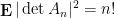
Van Vu and I have just uploaded to the arXiv our paper A central limit theorem for the determinant of a Wigner matrix, submitted to Adv. Math.. It studies the asymptotic distribution of the determinant {\det M_n} of a random Wigner matrix (such as a matrix drawn from the Gaussian Unitary Ensemble (GUE) or Gaussian Orthogonal Ensemble (GOE)).

Before we get to these results, let us first discuss the simpler problem of studying the determinant {\det A_n} of a random iid matrix {A_n = (\zeta_{ij})_{1 \leq i,j \leq n}}, such as a real gaussian matrix (where all entries are independently and identically distributed using the standard real normal distribution {\zeta_{ij} \equiv N(0,1)_{\bf R}}), a complex gaussian matrix (where all entries are independently and identically distributed using the standard complex normal distribution {\zeta_{ij} \equiv N(0,1)_{\bf C}}, thus the real and imaginary parts are independent with law {N(0,1/2)_{\bf R}}), or the random sign matrix (in which all entries are independently and identically distributed according to the Bernoulli distribution {\zeta_{ij} \equiv \pm 1} (with a {1/2} chance of either sign). More generally, one can consider a matrix {A_n} in which all the entries {\zeta_{ij}} are independently and identically distributed with mean zero and variance {1}.

We can expand {\det A_n} using the Leibniz expansion

\displaystyle  \det A_n = \sum_{\sigma \in S_n} I_\sigma, \ \ \ \ \ (1)

where {\sigma: \{1,\ldots,n\} \rightarrow \{1,\ldots,n\}} ranges over the permutations of {\{1,\ldots,n\}}, and {I_\sigma} is the product

\displaystyle  I_\sigma := \hbox{sgn}(\sigma) \prod_{i=1}^n \zeta_{i\sigma(i)}.

From the iid nature of the {\zeta_{ij}}, we easily see that each {I_\sigma} has mean zero and variance one, and are pairwise uncorrelated as {\sigma} varies. We conclude that {\det A_n} has mean zero and variance {n!} (an observation first made by Turán). In particular, from Chebyshev’s inequality we see that {\det A_n} is typically of size {O(\sqrt{n!})}.

It turns out, though, that this is not quite best possible. This is easiest to explain in the real gaussian case, by performing a computation first made by Goodman. In this case, {\det A_n} is clearly symmetrical, so we can focus attention on the magnitude {|\det A_n|}. We can interpret this quantity geometrically as the volume of an {n}-dimensional parallelopiped whose generating vectors {X_1,\ldots,X_n} are independent real gaussian vectors in {{\bf R}^n} (i.e. their coefficients are iid with law {N(0,1)_{\bf R}}). Using the classical base-times-height formula, we thus have

\displaystyle  |\det A_n| = \prod_{i=1}^n \hbox{dist}(X_i, V_i) \ \ \ \ \ (2)

where {V_i} is the {i-1}-dimensional linear subspace of {{\bf R}^n} spanned by {X_1,\ldots,X_{i-1}} (note that {X_1,\ldots,X_n}, having an absolutely continuous joint distribution, are almost surely linearly independent). Taking logarithms, we conclude

\displaystyle  \log |\det A_n| = \sum_{i=1}^n \log \hbox{dist}(X_i, V_i).

Now, we take advantage of a fundamental symmetry property of the Gaussian vector distribution, namely its invariance with respect to the orthogonal group {O(n)}. Because of this, we see that if we fix {X_1,\ldots,X_{i-1}} (and thus {V_i}, the random variable {\hbox{dist}(X_i,V_i)} has the same distribution as {\hbox{dist}(X_i,{\bf R}^{i-1})}, or equivalently the {\chi} distribution

\displaystyle  \chi_{n-i+1} := (\sum_{j=1}^{n-i+1} \xi_{n-i+1,j}^2)^{1/2}

where {\xi_{n-i+1,1},\ldots,\xi_{n-i+1,n-i+1}} are iid copies of {N(0,1)_{\bf R}}. As this distribution does not depend on the {X_1,\ldots,X_{i-1}}, we conclude that the law of {\log |\det A_n|} is given by the sum of {n} independent {\chi}-variables:

\displaystyle  \log |\det A_n| \equiv \sum_{j=1}^{n} \log \chi_j.

A standard computation shows that each {\chi_j^2} has mean {j} and variance {2j}, and then a Taylor series (or Ito calculus) computation (using concentration of measure tools to control tails) shows that {\log \chi_j} has mean {\frac{1}{2} \log j - \frac{1}{2j} + O(1/j^{3/2})} and variance {\frac{1}{2j}+O(1/j^{3/2})}. As such, {\log |\det A_n|} has mean {\frac{1}{2} \log n! - \frac{1}{2} \log n + O(1)} and variance {\frac{1}{2} \log n + O(1)}. Applying a suitable version of the central limit theorem, one obtains the asymptotic law

\displaystyle  \frac{\log |\det A_n| - \frac{1}{2} \log n! + \frac{1}{2} \log n}{\sqrt{\frac{1}{2}\log n}} \rightarrow N(0,1)_{\bf R}, \ \ \ \ \ (3)

where {\rightarrow} denotes convergence in distribution. A bit more informally, we have

\displaystyle  |\det A_n| \approx n^{-1/2} \sqrt{n!} \exp( N( 0, \log n / 2 )_{\bf R} ) \ \ \ \ \ (4)

when {A_n} is a real gaussian matrix; thus, for instance, the median value of {|\det A_n|} is {n^{-1/2+o(1)} \sqrt{n!}}. At first glance, this appears to conflict with the second moment bound {\mathop{\bf E} |\det A_n|^2 = n!} of Turán mentioned earlier, but once one recalls that {\exp(N(0,t)_{\bf R})} has a second moment of {\exp(2t)}, we see that the two facts are in fact perfectly consistent; the upper tail of the normal distribution in the exponent in (4) ends up dominating the second moment.

It turns out that the central limit theorem (3) is valid for any real iid matrix with mean zero, variance one, and an exponential decay condition on the entries; this was first claimed by Girko, though the arguments in that paper appear to be incomplete. Another proof of this result, with more quantitative bounds on the convergence rate has been recently obtained by Hoi Nguyen and Van Vu. The basic idea in these arguments is to express the sum in (2) in terms of a martingale and apply the martingale central limit theorem.

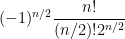
If one works with complex gaussian random matrices instead of real gaussian random matrices, the above computations change slightly (one has to replace the real {\chi} distribution with the complex {\chi} distribution, in which the {\xi_{i,j}} are distributed according to the complex gaussian {N(0,1)_{\bf C}} instead of the real one). At the end of the day, one ends up with the law

\displaystyle  \frac{\log |\det A_n| - \frac{1}{2} \log n! + \frac{1}{4} \log n}{\sqrt{\frac{1}{4}\log n}} \rightarrow N(0,1)_{\bf R}, \ \ \ \ \ (5)

or more informally

\displaystyle  |\det A_n| \approx n^{-1/4} \sqrt{n!} \exp( N( 0, \log n / 4 )_{\bf R} ) \ \ \ \ \ (6)

(but note that this new asymptotic is still consistent with Turán’s second moment calculation).

We can now turn to the results of our paper. Here, we replace the iid matrices
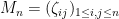
 {A_n} by Wigner matrices {M_n = (\zeta_{ij})_{1 \leq i,j \leq n}}, which are defined similarly but are constrained to be Hermitian (or real symmetric), thus {\zeta_{ij} = \overline{\zeta_{ji}}} for all {i,j}. Model examples here include the Gaussian Unitary Ensemble (GUE), in which {\zeta_{ij} \equiv N(0,1)_{\bf C}} for {1 \leq i < j \leq n} and {\zeta_{ij} \equiv N(0,1)_{\bf R}} for {1 \leq i=j \leq n}, the Gaussian Orthogonal Ensemble (GOE), in which {\zeta_{ij} \equiv N(0,1)_{\bf R}} for {1 \leq i < j \leq n} and {\zeta_{ij} \equiv N(0,2)_{\bf R}} for {1 \leq i=j \leq n}, and the symmetric Bernoulli ensemble, in which {\zeta_{ij} \equiv \pm 1} for {1 \leq i \leq j \leq n} (with probability {1/2} of either sign). In all cases, the upper triangular entries of the matrix are assumed to be jointly independent. For a more precise definition of the Wigner matrix ensembles we are considering, see the introduction to our paper.

The determinants {\det M_n} of these matrices still have a Leibniz expansion. However, in the Wigner case, the mean and variance of the {I_\sigma} are slightly different, and what is worse, they are not all pairwise uncorrelated any more. For instance, the mean of {I_\sigma} is still usually zero, but equals {(-1)^{n/2}} in the exceptional case when {\sigma} is a perfect matching (i.e. the union of exactly {n/2} {2}-cycles, a possibility that can of course only happen when {n} is even). As such, the mean {\mathop{\bf E} \det M_n} still vanishes when {n} is odd, but for even {n} it is equal to

\displaystyle  (-1)^{n/2} \frac{n!}{(n/2)!2^{n/2}}

(the fraction here simply being the number of perfect matchings on {n} vertices). Using Stirling’s formula, one then computes that {|\mathop{\bf E} \det A_n|} is comparable to {n^{-1/4} \sqrt{n!}} when {n} is large and even. The second moment calculation is more complicated (and uses facts about the distribution of cycles in random permutations, mentioned in this previous post), but one can compute that {\mathop{\bf E} |\det A_n|^2} is comparable to {n^{1/2} n!} for GUE and {n^{3/2} n!} for GOE. (The discrepancy here comes from the fact that in the GOE case, {I_\sigma} and {I_\rho} can correlate when {\rho} contains reversals of {k}-cycles of {\sigma} for {k \geq 3}, but this does not happen in the GUE case.) For GUE, much more precise asymptotics for the moments of the determinant are known, starting from the work of Brezin and Hikami, though we do not need these more sophisticated computations here.

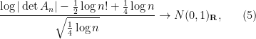
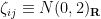
Our main results are then as follows.

Theorem 1 Let {M_n} be a Wigner matrix.

  • If {M_n} is drawn from GUE, then

    \displaystyle  \frac{\log |\det M_n| - \frac{1}{2} \log n! + \frac{1}{4} \log n}{\sqrt{\frac{1}{2}\log n}} \rightarrow N(0,1)_{\bf R}.

  • If {M_n} is drawn from GOE, then

    \displaystyle  \frac{\log |\det M_n| - \frac{1}{2} \log n! + \frac{1}{4} \log n}{\sqrt{\log n}} \rightarrow N(0,1)_{\bf R}.

  • The previous two results also hold for more general Wigner matrices, assuming that the real and imaginary parts are independent, a finite moment condition is satisfied, and the entries match moments with those of GOE or GUE to fourth order. (See the paper for a more precise formulation of the result.)

Thus, we informally have

\displaystyle  |\det M_n| \approx n^{-1/4} \sqrt{n!} \exp( N( 0, \log n / 2 )_{\bf R} )

when {M_n} is drawn from GUE, or from another Wigner ensemble matching GUE to fourth order (and obeying some additional minor technical hypotheses); and

\displaystyle  |\det M_n| \approx n^{-1/4} \sqrt{n!} \exp( N( 0, \log n )_{\bf R} )

when {M_n} is drawn from GOE, or from another Wigner ensemble matching GOE to fourth order. Again, these asymptotic limiting distributions are consistent with the asymptotic behaviour for the second moments.

The extension from the GUE or GOE case to more general Wigner ensembles is a fairly routine application of the four moment theorem for Wigner matrices, although for various technical reasons we do not quite use the existing four moment theorems in the literature, but adapt them to the log determinant. The main idea is to express the log-determinant as an integral

\displaystyle  \log|\det M_n| = \frac{1}{2} n \log n - n \hbox{Im} \int_0^\infty s(\sqrt{-1}\eta)\ d\eta \ \ \ \ \ (7)

of the Stieltjes transform
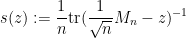
\displaystyle  s(z) := \frac{1}{n} \hbox{tr}( \frac{1}{\sqrt{n}} M_n - z )^{-1}

of {M_n}. Strictly speaking, the integral in (7) is divergent at infinity (and also can be ill-behaved near zero), but this can be addressed by standard truncation and renormalisation arguments (combined with known facts about the least singular value of Wigner matrices), which we omit here. We then use a variant of the four moment theorem for the Stieltjes transform, as used by Erdos, Yau, and Yin (based on a previous four moment theorem for individual eigenvalues introduced by Van Vu and myself). The four moment theorem is proven by the now-standard Lindeberg exchange method, combined with the usual resolvent identities to control the behaviour of the resolvent (and hence the Stieltjes transform) with respect to modifying one or two entries, together with the delocalisation of eigenvector property (which in turn arises from local semicircle laws) to control the error terms.

Somewhat surprisingly (to us, at least), it turned out that it was the first part of the theorem (namely, the verification of the limiting law for the invariant ensembles GUE and GOE) that was more difficult than the extension to the Wigner case. Even in an ensemble as highly symmetric as GUE, the rows are no longer independent, and the formula (2) is basically useless for getting any non-trivial control on the log determinant. There is an explicit formula for the joint distribution of the eigenvalues of GUE (or GOE), which does eventually give the distribution of the cumulants of the log determinant, which then gives the required central limit theorem; but this is a lengthy computation, first performed by Delannay and Le Caer.

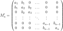
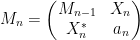
Following a suggestion of my colleague, Rowan Killip, we give an alternate proof of this central limit theorem in the GUE and GOE cases, by using a beautiful observation of Trotter, namely that the GUE or GOE ensemble can be conjugated into a tractable tridiagonal form. Let me state it just for GUE:

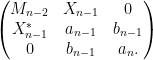
Proposition 2 (Tridiagonal form of GUE) Let {M'_n} be the random tridiagonal real symmetric matrix
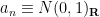
\displaystyle  M'_n = \begin{pmatrix} a_1 & b_1 & 0 & \ldots & 0 & 0 \\ b_1 & a_2 & b_2 & \ldots & 0 & 0 \\ 0 & b_2 & a_3 & \ldots & 0 & 0 \\ \vdots & \vdots & \vdots & \ddots & \vdots & \vdots \\ 0 & 0 & 0 & \ldots & a_{n-1} & b_{n-1} \\ 0 & 0 & 0 & \ldots & b_{n-1} & a_n \end{pmatrix}

where the {a_1,\ldots,a_n, b_1,\ldots,b_{n-1}} are jointly independent real random variables, with {a_1,\ldots,a_n \equiv N(0,1)_{\bf R}} being standard real Gaussians, and each {b_i} having a {\chi}-distribution:

\displaystyle  b_i = (\sum_{j=1}^i |z_{i,j}|^2)^{1/2}

where {z_{i,j} \equiv N(0,1)_{\bf C}} are iid complex gaussians. Let {M_n} be drawn from GUE. Then the joint eigenvalue distribution of {M_n} is identical to the joint eigenvalue distribution of {M'_n}.

Proof: Let {M_n} be drawn from GUE. We can write

\displaystyle  M_n = \begin{pmatrix} M_{n-1} & X_n \\ X_n^* & a_n \end{pmatrix}

where {M_{n-1}} is drawn from the {n-1\times n-1} GUE, {a_n \equiv N(0,1)_{\bf R}}, and {X_n \in {\bf C}^{n-1}} is a random gaussian vector with all entries iid with distribution {N(0,1)_{\bf C}}. Furthermore, {M_{n-1}, X_n, a_n} are jointly independent.

We now apply the tridiagonal matrix algorithm. Let {b_{n-1} := |X_n|}, then {b_n} has the {\chi}-distribution indicated in the proposition. We then conjugate {M_n} by a unitary matrix {U} that preserves the final basis vector {e_n}, and maps {X} to {b_{n-1} e_{n-1}}. Then we have

\displaystyle  U M_n U^* = \begin{pmatrix} \tilde M_{n-1} & b_{n-1} e_{n-1} \\ b_{n-1} e_{n-1}^* & a_n \end{pmatrix}

where {\tilde M_{n-1}} is conjugate to {M_{n-1}}. Now we make the crucial observation: because {M_{n-1}} is distributed according to GUE (which is a unitarily invariant ensemble), and {U} is a unitary matrix independent of {M_{n-1}}, {\tilde M_{n-1}} is also distributed according to GUE, and remains independent of both {b_{n-1}} and {a_n}.

We continue this process, expanding {U M_n U^*} as

\displaystyle \begin{pmatrix} M_{n-2} & X_{n-1} & 0 \\ X_{n-1}^* & a_{n-1} & b_{n-1} \\ 0 & b_{n-1} & a_n. \end{pmatrix}

Applying a further unitary conjugation that fixes {e_{n-1}, e_n} but maps {X_{n-1}} to {b_{n-2} e_{n-2}}, we may replace {X_{n-1}} by {b_{n-2} e_{n-2}} while transforming {M_{n-2}} to another GUE matrix {\tilde M_{n-2}} independent of {a_n, b_{n-1}, a_{n-1}, b_{n-2}}. Iterating this process, we eventually obtain a coupling of {M_n} to {M'_n} by unitary conjugations, and the claim follows. \Box

The determinant of a tridiagonal matrix is not quite as simple as the determinant of a triangular matrix (in which it is simply the product of the diagonal entries), but it is pretty close: the determinant {D_n} of the above matrix is given by solving the recursion

\displaystyle  D_i = a_i D_{i-1} + b_{i-1}^2 D_{i-2}

with {D_0=1} and {D_{-1} = 0}. Thus, instead of the product of a sequence of independent scalar {\chi} distributions as in the gaussian matrix case, the determinant of GUE ends up being controlled by the product of a sequence of independent {2\times 2} matrices whose entries are given by gaussians and {\chi} distributions. In this case, one cannot immediately take logarithms and hope to get something for which the martingale central limit theorem can be applied, but some ad hoc manipulation of these {2 \times 2} matrix products eventually does make this strategy work. (Roughly speaking, one has to work with the logarithm of the Frobenius norm of the matrix first.)

In the Winter quarter (starting on January 9), I will be teaching a graduate course on expansion in groups of Lie type.  This course will focus on constructions of expanding Cayley graphs on finite groups of Lie type (such as the special linear groups SL_d({\bf F}_q), or their simple quotients PSL_d({\bf F}_q), but also including more exotic “twisted” groups of Lie type, such as the Steinberg or Suzuki-Ree groups), including the “classical” constructions of Margulis and of Selberg, but also the more recent constructions of Bourgain-Gamburd and later authors (including some very recent work of Ben Green, Emmanuel Breuillard, Rob Guralnick, and myself which is nearing completion and which I plan to post about shortly).  As usual, I plan to start posting lecture notes on this blog before the course begins.

Archives