LLet {L: H \rightarrow H} be a self-adjoint operator on a finite-dimensional Hilbert space {H}. The behaviour of this operator can be completely described by the spectral theorem for finite-dimensional self-adjoint operators (i.e. Hermitian matrices, when viewed in coordinates), which provides a sequence {\lambda_1,\ldots,\lambda_n \in {\bf R}} of eigenvalues and an orthonormal basis {e_1,\ldots,e_n} of eigenfunctions such that {L e_i = \lambda_i e_i} for all {i=1,\ldots,n}. In particular, given any function {m: \sigma(L) \rightarrow {\bf C}} on the spectrum {\sigma(L) := \{ \lambda_1,\ldots,\lambda_n\}} of {L}, one can then define the linear operator {m(L): H \rightarrow H} by the formula

\displaystyle m(L) e_i := m(\lambda_i) e_i,

which then gives a functional calculus, in the sense that the map {m \mapsto m(L)} is a {C^*}-algebra isometric homomorphism from the algebra {BC(\sigma(L) \rightarrow {\bf C})} of bounded continuous functions from {\sigma(L)} to {{\bf C}}, to the algebra {B(H \rightarrow H)} of bounded linear operators on {H}. Thus, for instance, one can define heat operators {e^{-tL}} for {t>0}, Schrödinger operators {e^{itL}} for {t \in {\bf R}}, resolvents {\frac{1}{L-z}} for {z \not \in \sigma(L)}, and (if {L} is positive) wave operators {e^{it\sqrt{L}}} for {t \in {\bf R}}. These will be bounded operators (and, in the case of the Schrödinger and wave operators, unitary operators, and in the case of the heat operators with {L} positive, they will be contractions). Among other things, this functional calculus can then be used to solve differential equations such as the heat equation

\displaystyle u_t + Lu = 0; \quad u(0) = f \ \ \ \ \ (1)


the Schrödinger equation

\displaystyle u_t + iLu = 0; \quad u(0) = f \ \ \ \ \ (2)


the wave equation

\displaystyle u_{tt} + Lu = 0; \quad u(0) = f; \quad u_t(0) = g \ \ \ \ \ (3)


or the Helmholtz equation

\displaystyle (L-z) u = f. \ \ \ \ \ (4)


The functional calculus can also be associated to a spectral measure. Indeed, for any vectors {f, g \in H}, there is a complex measure {\mu_{f,g}} on {\sigma(L)} with the property that

\displaystyle \langle m(L) f, g \rangle_H = \int_{\sigma(L)} m(x) d\mu_{f,g}(x);

indeed, one can set {\mu_{f,g}} to be the discrete measure on {\sigma(L)} defined by the formula

\displaystyle \mu_{f,g}(E) := \sum_{i: \lambda_i \in E} \langle f, e_i \rangle_H \langle e_i, g \rangle_H.

One can also view this complex measure as a coefficient

\displaystyle \mu_{f,g} = \langle \mu f, g \rangle_H

of a projection-valued measure {\mu} on {\sigma(L)}, defined by setting

\displaystyle \mu(E) f := \sum_{i: \lambda_i \in E} \langle f, e_i \rangle_H e_i.

Finally, one can view {L} as unitarily equivalent to a multiplication operator {M: f \mapsto g f} on {\ell^2(\{1,\ldots,n\})}, where {g} is the real-valued function {g(i) := \lambda_i}, and the intertwining map {U: \ell^2(\{1,\ldots,n\}) \rightarrow H} is given by

\displaystyle U ( (c_i)_{i=1}^n ) := \sum_{i=1}^n c_i e_i,

so that {L = U M U^{-1}}.

It is an important fact in analysis that many of these above assertions extend to operators on an infinite-dimensional Hilbert space {H}, so long as one one is careful about what “self-adjoint operator” means; these facts are collectively referred to as the spectral theorem. For instance, it turns out that most of the above claims have analogues for bounded self-adjoint operators {L: H \rightarrow H}. However, in the theory of partial differential equations, one often needs to apply the spectral theorem to unbounded, densely defined linear operators {L: D \rightarrow H}, which (initially, at least), are only defined on a dense subspace {D} of the Hilbert space {H}. A very typical situation arises when {H = L^2(\Omega)} is the square-integrable functions on some domain or manifold {\Omega} (which may have a boundary or be otherwise “incomplete”), and {D = C^\infty_c(\Omega)} are the smooth compactly supported functions on {\Omega}, and {L} is some linear differential operator. It is then of interest to obtain the spectral theorem for such operators, so that one build operators such as {e^{-tL}, e^{itL}, \frac{1}{L-z}, e^{it\sqrt{L}}} or to solve equations such as (1), (2), (3), (4).

In order to do this, some necessary conditions on the densely defined operator {L: D \rightarrow H} must be imposed. The most obvious is that of symmetry, which asserts that

\displaystyle \langle Lf, g \rangle_H = \langle f, Lg \rangle_H \ \ \ \ \ (5)


for all {f, g \in D}. In some applications, one also wants to impose positive definiteness, which asserts that

\displaystyle \langle Lf, f \rangle_H \geq 0 \ \ \ \ \ (6)


for all {f \in D}. These hypotheses are sufficient in the case when {L} is bounded, and in particular when {H} is finite dimensional. However, as it turns out, for unbounded operators these conditions are not, by themselves, enough to obtain a good spectral theory. For instance, one consequence of the spectral theorem should be that the resolvents {(L-z)^{-1}} are well-defined for any strictly complex {z}, which by duality implies that the image of {L-z} should be dense in {H}. However, this can fail if one just assumes symmetry, or symmetry and positive definiteness. A well-known example occurs when {H} is the Hilbert space {H := L^2((0,1))}, {D := C^\infty_c((0,1))} is the space of test functions, and {L} is the one-dimensional Laplacian {L := -\frac{d^2}{dx^2}}. Then {L} is symmetric and positive, but the operator {L-k^2} does not have dense image for any complex {k}, since

\displaystyle \langle (L-\overline{k}^2) f, e^{\overline{k}x} \rangle_H = 0

for all test functions {f \in C^\infty_c((0,1))}, as can be seen from a routine integration by parts. As such, the resolvent map is not everywhere uniquely defined. There is also a lack of uniqueness for the wave, heat, and Schrödinger equations for this operator (note that there are no spatial boundary conditions specified in these equations).

Another example occurs when {H := L^2((0,+\infty))}, {D := C^\infty_c((0,+\infty))}, {L} is the momentum operator {L := i \frac{d}{dx}}. Then the resolvent {(L-z)^{-1}} can be uniquely defined for {z} in the upper half-plane, but not in the lower half-plane, due to the obstruction

\displaystyle \langle (L-z) f, e^{i \bar{z} x} \rangle_H = 0

for all test functions {f} (note that the function {e^{i\bar{z} x}} lies in {L^2((0,+\infty))} when {z} is in the lower half-plane). For related reasons, the translation operators {e^{itL}} have a problem with either uniqueness or existence (depending on whether {t} is positive or negative), due to the unspecified boundary behaviour at the origin.

The key property that lets one avoid this bad behaviour is that of essential self-adjointness. Once {L} is essentially self-adjoint, then spectral theorem becomes applicable again, leading to all the expected behaviour (e.g. existence and uniqueness for the various PDE given above).

Unfortunately, the concept of essential self-adjointness is defined rather abstractly, and is difficult to verify directly; unlike the symmetry condition (5) or the positive condition (6), it is not a “local” condition that can be easily verified just by testing {L} on various inputs, but is instead a more “global” condition. In practice, to verify this property, one needs to invoke one of a number of a partial converses to the spectral theorem, which roughly speaking asserts that if at least one of the expected consequences of the spectral theorem is true for some symmetric densely defined operator {L}, then {L} is self-adjoint. Examples of “expected consequences” include:

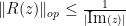
  • Existence of resolvents {(L-z)^{-1}} (or equivalently, dense image for {L-z});
  • Existence of a contractive heat propagator semigroup {e^{tL}} (in the positive case);
  • Existence of a unitary Schrödinger propagator group {e^{itL}};
  • Existence of a unitary wave propagator group {e^{it\sqrt{L}}} (in the positive case);
  • Existence of a “reasonable” functional calculus.
  • Unitary equivalence with a multiplication operator.

Thus, to actually verify essential self-adjointness of a differential operator, one typically has to first solve a PDE (such as the wave, Schrödinger, heat, or Helmholtz equation) by some non-spectral method (e.g. by a contraction mapping argument, or a perturbation argument based on an operator already known to be essentially self-adjoint). Once one can solve one of the PDEs, then one can apply one of the known converse spectral theorems to obtain essential self-adjointness, and then by the forward spectral theorem one can then solve all the other PDEs as well. But there is no getting out of that first step, which requires some input (typically of an ODE, PDE, or geometric nature) that is external to what abstract spectral theory can provide. For instance, if one wants to establish essential self-adjointness of the Laplace-Beltrami operator {L = -\Delta_g} on a smooth Riemannian manifold {(M,g)} (using {C^\infty_c(M)} as the domain space), it turns out (under reasonable regularity hypotheses) that essential self-adjointness is equivalent to geodesic completeness of the manifold, which is a global ODE condition rather than a local one: one needs geodesics to continue indefinitely in order to be able to (unitarily) solve PDEs such as the wave equation, which in turn leads to essential self-adjointness. (Note that the domains {(0,1)} and {(0,+\infty)} in the previous examples were not geodesically complete.) For this reason, essential self-adjointness of a differential operator is sometimes referred to as quantum completeness (with the completeness of the associated Hamilton-Jacobi flow then being the analogous classical completeness).

In these notes, I wanted to record (mostly for my own benefit) the forward and converse spectral theorems, and to verify essential self-adjointness of the Laplace-Beltrami operator on geodesically complete manifolds. This is extremely standard analysis (covered, for instance, in the texts of Reed and Simon), but I wanted to write it down myself to make sure that I really understood this foundational material properly.

— 1. Self-adjointness and resolvents —

To begin, we study what we can abstractly say about a densely defined symmetric linear operator {L: D \rightarrow H} on a Hilbert space {H}. To avoid some technical issues we shall assume that the Hilbert space is separable, which is the case typically encountered in applications (particularly in PDE). We will occasionally assume also that {L} is positive, but will make this hypothesis explicit whenever we are doing so.

All convergence in Hilbert spaces will be in the strong (i.e. norm) topology unless otherwise stated. Similarly, all inner products and norms will be over {H} unless otherwise stated.

For technical reasons, it is convenient to reduce to the case when {L} is closed, which means that the graph {\{ (f, Lf): f \in D \}} is a closed subspace of {H \times H}. Equivalently, {L} is closed if whenever {f_n \in D} is a sequence converging strongly to a limit {f \in H}, and {Lf_n} converges to a limit {g} in {H}, then {f \in D} and {g = Lf}. For instance, thanks to the closed graph theorem, an everywhere-defined linear operator is closed if and only if it is bounded.

Not every densely defined symmetric linear operator is closed (indeed, one could take a closed operator and restrict the domain of definition to a proper dense subspace). However, all such operators are closable, in that they have a closure:

Lemma 1 (Closure) Let {L: D \rightarrow H} be a densely defined symmetric linear operator. Then there exists a unique extension {\overline{L}: \overline{D} \rightarrow H} of {L} as a closed, densely defined symmetric linear operator, such that the graph {\{ (f, \overline{L} f): f \in \overline{D} \}} of {\overline{L}} is the closure of the graph {\{ (f, Lf): f \in D \}} of {L}.

Proof: The key step is to show that the closure {\overline{\{ (f, Lf): f \in D \}}} of the graph of {L} remains a graph, i.e. it obeys the vertical line test. If this failed, then by linearity one could find a sequence {f_n \in D} converging to zero such that {Lf_n} converged to a non-zero limit {g}. Since {D} is dense, we can find {g' \in D} such that {\langle g, g' \rangle \neq 0}. But then by symmetry

\displaystyle \langle f_n, Lg' \rangle = \langle Lf_n, g' \rangle = \langle g_n, g' \rangle \rightarrow \langle g, g' \rangle \neq 0.

On the other hand, as {f_n \rightarrow 0}, {\langle f_n, Lg' \rangle \rightarrow 0}. Thus {\overline{\{ (f, Lf): f \in D \}}} is the graph of some function {\overline{L}: \overline{D} \rightarrow H}. It is easy to see that this is a densely defined symmetric linear operator extending {L}, and is the unique such operator. \Box

Exercise 1 Show that {\overline{L}} is positive if and only if {L} is positive.

Remark 1 We caution that {\overline{D}} is not the closure or completion of {D} with respect to the usual norm {f \mapsto \|f\|} on {D}. (Indeed, as {D} is a dense subspace of {H}, that completion of {D} is simply {H}.) However, it is the completion of {D} with respect to the modified norm {f \mapsto \|f\| + \|Lf\|}.

In PDE applications, the closure {\overline{L}} tends to be defined on a Sobolev space of functions that behave well at the boundary, and is given by a distributional derivative. Here is a simple example of this:

Exercise 2 Let {L} be the Laplacian {L = -\frac{d^2}{dx^2}}, defined on the dense subspace {D := C^\infty_c((0,1))} of {H := L^2((0,1))}. Show that the closure {\overline{L}} is defined on the Sobolev space {H^2_0((0,1))}, defined as the completion of {C^\infty_c((0,1))} under the Sobolev norm

\displaystyle \|f\|_{H^2_0((0,1))} := \| f \|_{L^2((0,1))} + \| Lf \|_{L^2((0,1))},

and that the action of {\overline{L}} is given by the weak (distributional) derivative, {\overline{L} = -\frac{d^2}{dx^2}}.

Next, we define the adjoint {L^*: D^* \rightarrow H} of {L: D \rightarrow H}, which informally speaking is the maximally defined operator for which one has the relationship

\displaystyle \langle Lf, g \rangle = \langle f, L^* g \rangle \ \ \ \ \ (7)


for {f \in D} and {g \in D^*}. More formally, define {D^*} to be the set of all vectors {g \in H} for which the map {f \mapsto \langle Lf, g \rangle} is a bounded linear functional on {D}, which thus extends to the closure {H} of {D}. For such {g \in H}, we may apply the Riesz representation theorem for Hilbert spaces and locate a unique vector {L^* g \in H} for which (7) holds. This is easily seen to define a linear operator {L^*: D^* \rightarrow H}. Furthermore, the claim that {L} is symmetric can be reformulated as the claim that {L^*} extends {L}.

If {L} is not symmetric, then {L^*} does not extend {L}, and need not be densely defined at all. However, it is still closed:

Exercise 3 Let {L: D \rightarrow H} be a densely defined linear operator, and let {L^*: D^* \rightarrow H} be its adjoint. Show that {\{ (-L^* g, g): g \in D^* \}} is the orthogonal complement in {H \times H} of (the closure of) {\{ (f, Lf): f \in D \}}. Conclude that {L^*} is always closed.

If {L} is symmetric, show that {L^{**} = \overline{L}} and {L^* = (\overline{L})^*}.

Exercise 4 Construct an example of a densely defined linear operator {L: D \rightarrow H} in a separable Hilbert space {H} for which {L^*} is only defined at {\{0\}}. (Hint: Build a dense linearly independent basis of {H}, let {D} be the algebraic span of that basis, and design {L} so that the graph of {L} is dense in {H \times H}.)

We caution that the adjoint {L^*: D^* \rightarrow H} of a symmetric densely defined operator {L: D \rightarrow H} need not be itself symmetric, despite extending the symmetric operator {L}:

Exercise 5 We continue Example 2. Show that for any complex number {k}, the functions {x \mapsto e^{kx}} lie in {D^*} with {L^* e^{kx} = -k^2 e^{kx}}. Deduce that {L^*} is not symmetric, and not positive.

Intuitively, the problem here is that the domain of {L} is too “small” (it stays too far away from the boundary), which makes the domain of {L^*} too “large” (it contains too much stuff coming from the boundary), which ruins the integration by parts argument that gives symmetry.

Now we can define (essential) self-adjointness.

Definition 2 Let {L: D \rightarrow H } be a densely defined linear operator.

  • {L} is self-adjoint if {L = L^*}. (Note that this implies in particular that {L} is symmetric and closed.)
  • {L} is essentially self-adjoint if it is symmetric, and its closure {\overline{L}} is self-adjoint.

Note that this extends the usual definition of self-adjointness for bounded operators. Conversely, from the closed graph theorem we also observe the Hellinger-Toeplitz theorem: an operator that is self-adjoint and everywhere defined, is necessarily bounded.

Exercise 6 Let {L: D \rightarrow H } be a densely defined symmetric closed linear operator. Show that {L} is self-adjoint if and only if {L^*} is symmetric.

It is not immediately obvious what advantage self-adjointness gives. To see this, we consider the problem of inverting the operator {L-z: D \rightarrow H} for some complex number {z}, where {L: D \rightarrow H} is densely defined, symmetric, and closed. Observe that if {f \in D}, then {\langle Lf, f \rangle = \langle f, Lf \rangle} is necessarily real. In particular,

\displaystyle \hbox{Im} \langle (L-z)f, f \rangle = - \hbox{Im} z \|f\|^2

and hence by the Cauchy-Schwarz inequality

\displaystyle \|(L-z) f \| \geq |\hbox{Im} z| \|f\|. \ \ \ \ \ (8)


In particular, if {z} is strictly complex (i.e. not real), then {L-z} is injective. Furthermore, we see that if {f_n \in D} is such that {(L-z) f_n} is convergent, then by (8) {f_n} is convergent also, and hence {Lf_n} is convergent. As {L} was assumed to be closed, we conclude that {f_n} converges to a limit {f} in {D}, and {(L-z)f_n} converges to {(L-z) f}. As a consequence, we see that the space {\hbox{Image}(L-z) := \{ (L-z)f: f \in D \}} is a closed subspace of {H}. From (8) we then see that we can define an inverse {R(z): \hbox{Image}(L-z) \rightarrow D} of {L-z}, which we call the resolvent of {L} with spectral parameter {z}; this is a bounded linear operator with norm {\|R(z)\|_{op} \leq \frac{1}{|\hbox{Im}(z)|}}.

Exercise 7 If {L} is densely defined, symmetric, closed, and positive, and {z} is a complex number with {\hbox{Re}(z) < 0}, show {R(z)} is well-defined on {\hbox{Image}(L-z)} with {\|R(z)\|_{op} \leq \frac{1}{|\hbox{Re}(z)|}}.

Now we observe a connection between self-adjointness and the domain of the resolvent. We first need some basic properties of the resolvent:

Exercise 8 Let {L: D \rightarrow H} be densely defined, symmetric, and closed.

  • (i) (Resolvent identity) If {z, w} are distinct strictly complex numbers with {R(z), R(w)} everywhere defined, show that {(z-w) R(z) R(w) = R(z) - R(w)}. (Hint: compute {R(z) (H-w) R(w) - R(z) (H-z) R(w)} two different ways.)
  • (ii) If {z} is a strictly complex number with {R(z)} and {R(z^*)} everywhere defined, show that {R(z)^* = R(z^*)}.

Proposition 3 Let {L: D \rightarrow H} be densely defined, symmetric, and closed, let {L^*: D^* \rightarrow H} be the adjoint, and let {z} be strictly complex.

  • (i) (Surjectivity is dual to injectivity) {R(z)} is everywhere defined if and only if the operator {L^* - z^*: D^* \rightarrow H} has trivial kernel.
  • (ii) (Self-adjointness implies surjectivity) If {L} is self-adjoint, then {R(z)} is everywhere defined.
  • (iii) (Surjectivity implies self-adjointness) Conversely, if {R(z)} and {R(z^*)} are both everywhere defined, then {L} is self-adjoint.

In particular, we see that we have a criterion for self-adjointness: a densely defined symmetric closed operator is self-adjoint if and only if {R(i)} and {R(-i)} are both everywhere defined, or in other words if {L+i} and {L-i} are both surjective.

Proof: We first prove (i). If {R(z)} is not everywhere defined, then the closed subspace {\hbox{Image}(L-z) \subset H} is not all of {H}. Thus there must be a non-zero vector {v \in H} in the orthogonal complement of this subspace, thus {\langle (L-z) f, g \rangle = 0} for all {f \in D}. In particular,

\displaystyle |\langle L f, g \rangle| = |z| |\langle f, g \rangle| \leq |z| \|f\| \|g\|

and hence, by definition of {D^*}, {g} lies in {D^*}. Now from (7) we have

\displaystyle \langle f, (L^* - z^*)g \rangle = \langle (L-z) f, g \rangle = 0

for all {f \in D}; since {D} is dense, we have {(L^* - z^*)g = 0} as required. The converse implication follows by reversing these steps.

Now we prove (ii). Suppose that {R(z)} was not everywhere defined. By (i) and self-adjointness, we conclude that {(L-z^*)f = 0} for some non-zero {f \in D}. But this contradicts (8).

Now we prove (iii). Let {g \in D^*}; our task is to show that {g \in D}. From Exercise 8(ii) and (7) one has

\displaystyle \langle f, R(z^*) (L^*-z^*) g \rangle = \langle R(z) f, (L^*-z^*) g \rangle = \langle (L-z) R(z) f, g \rangle = \langle f, g \rangle

for all {f \in H}. We conclude that {g = R(z^*) (L^*-z^*) g}. Since {R(z^*)} takes values in {D}, the claim follows. \Box

Exercise 9 Let {L: D \rightarrow H} be densely defined, symmetric, and closed, and let {z} be strictly complex.

  • (i) If {R(z)} is everywhere defined, show that {R(w)} is everywhere defined whenever {|w-z| < \hbox{Im}(z)}. (Hint: use Neumann series.)
  • (ii) If {R(z)} is everywhere defined, show that {R(w)} is everywhere defined whenever {\hbox{Im}(w)} has the same sign as {\hbox{Im}(z)}.
  • (iii) If {L} is positive, and {w} is not a non-negative real, show that {R(w)} is everywhere defined if and only if {L} is self-adjoint.

As a particular corollary of the above exercise, we see that a densely defined, symmetric closed positive operator {L} is self-adjoint if and only if {R(-1)} is everywhere defined, or in other words if {1+L} is surjective.

Exercise 10 Let {(X,\mu)} be a measure space with a countably generated {\sigma}-algebra (so that {L^2(X,\mu)} is separable), let {m: X \rightarrow {\bf R}} be a measurable function, and let {D} be the space of all {f \in L^2(X,\mu)} such that {mf \in L^2(X,\mu)}. Show that the multiplier operator {L: D \rightarrow L^2(X,\mu)} defined by {L f := mf} is a densely defined self-adjoint operator.

Exercise 11 Let {H := L^2((0,+\infty))}, {D := C^\infty_c((0,+\infty))}, and {L} is the momentum operator {L := i \frac{d}{dx}}. Show that {L} is densely defined and symmetric, and {R(-i)} is everywhere defined, but {R(i)} is only defined on the orthogonal complement of {e^{-x}}. (Here, we define the resolvent of a closable operator to be the resolvent of its closure.) In particular, {L} is not self-adjoint.

Exercise 12 Let {L} be densely defined and symmetric.

  • (i) Show that {L} is essentially self-adjoint if and only if {\hbox{Image}(L+i)} and {\hbox{Image}(L-i)} are dense in {H}.
  • (ii) If {L} is positive, show that {L} is essentially self-adjoint if and only if {\hbox{Image}(1+L)} is dense in {H}.

Exercise 13 Let {a_1, a_2, \ldots} and {b_1,b_2,\ldots} be sequences of real numbers, with the {b_n} all non-zero. Define the Jacobi operator {T: \ell^2_c({\bf N}) \rightarrow \ell^2({\bf N})} from the space {\ell^2_c({\bf N})} of compactly supported sequences {(x_n)_{n=1}^\infty} to the space {\ell^2({\bf N})} of square-summable sequences {(y_n)_{n=1}^\infty} by the formula

\displaystyle T (x_n)_{n=1}^\infty = (b_{n-1} x_{n-1} + a_n x_n + b_n x_{n+1})_{n=1}^\infty

with the convention that {b_{n-1} x_{n-1}} vanishes for {n=1}.

  • (i) Show that {T} is densely defined and symmetric.
  • (ii) Show that {T} is essentially self-adjoint if and only if the (unique) solution {\phi_n} to the recurrence

    \displaystyle b_{n-1} \phi_{n-1} + (a_n-i) \phi_n + b_n \phi_{n+1} = 0

    with {\phi_1 = 1} (and the convention {b_0\phi_0=0}), is not square-summable.

This exercise shows that the self-adjointness of an operator, even one as explicit as a Jacobi operator, can depend in a rather subtle and “global” fashion on the behaviour of the coefficients of that oeprator.

— 2. Self-adjointness and spectral measure —

We have seen that self-adjoint operators have everywhere-defined resolvents {R(z)} for all strictly complex {z}. Now we use this fact to build spectral measures. We will need a useful tool from complex analysis, which places a one-to-one correspondence between finite non-negative measures on {{\bf R}} and certain analytic functions on the upper half-plane:

Theorem 4 (Herglotz representation theorem) Let {F: {\bf H} \rightarrow \overline{{\bf H}}} be an analytic function from the upper half-plane {{\bf H} := \{ z \in {\bf C}: \hbox{Im}(z) > 0 \}} to the closed upper half-plane {\overline{{\bf H}} := \{ z \in {\bf C}: \hbox{Im}(z) \geq 0 \}}, obeying a bound of the form {|F(z)| \leq C / \hbox{Im}(z)} for all {z \in {\bf H}} and some {C>0}. Then there exists a finite non-negative Radon measure {\mu} on {{\bf R}} such that

\displaystyle F(z) = \int_{\bf R} \frac{1}{x-z}\ d\mu(x) \ \ \ \ \ (9)


for all {z \in {\bf H}}. Furthermore, one has {y F(iy) \rightarrow \mu({\bf R})} as {y \rightarrow +\infty}.

We set the proof of the above theorem as an exercise below. Note in the converse direction that if {\mu} is a finite non-negative Radon measure, then the function {F} defined by (9) obeys all the hypotheses of the theorem. The Herglotz representation theorem, like the more well known Riesz representation theorem for measures, is a useful tool to construct non-negative Radon measures; later on we will also use Bochner’s theorem for a similar purpose.

Exercise 14 Let {F} be as in the hypothesis of the Herglotz representation theorem. For each {\epsilon > 0}, let {F_\epsilon: {\bf R} \rightarrow \overline{{\bf H}}} be the function {F_\epsilon(x) := F(x+i\epsilon)}.

  • (i) Show that one has {F_{\epsilon+t} = F_\epsilon * P_t} for all {\epsilon, t > 0}, where {P_t(x) := \frac{1}{\pi} \frac{t}{x^2+t^2}} is the Poisson kernel and {*} is the usual convolution operation.
  • (ii) Show that the non-negative measures {\hbox{Im} F_\epsilon(x)\ dx} have a finite mass independent of {\epsilon}, and converge in the vague topology as {\epsilon \rightarrow 0} to a non-negative finite measure {\mu}.
  • (iii) Prove the Herglotz representation theorem.

Now we return to spectral theory. Let {L: D \rightarrow H} be a densely-defined self-adjoint operator, and let {f \in H}. We consider the function

\displaystyle F_{f,f}(z) := \langle R(z) f, f \rangle

on the upper half-plane. We can use this function and the Herglotz representation theorem to construct spectral measures {\mu_{f,f}}:

Exercise 15 Let {L}, {f}, and {F_{f,f}} be as above.

  • (i) Show that {F_{f,f}} is analytic. (Hint: use Neumann series and Morera’s theorem.)
  • (ii) Show that {|F_{f,f}(z)| \leq \|f\|^2/\hbox{Im}(z)} for all {z} in the upper half-plane.
  • (iii) Show that {\hbox{Im} F_{f,f}(z) \geq 0} for all {z} in the upper half-plane. (Hint: You will find Exercise 8 to be useful.)
  • (iv) Show that {iy F_{f,f}(iy) \rightarrow \|f\|^2} for all {f \in H}. (Hint: first show this for {f \in D}, writing {f = R(i) g} for some {g \in H}.)
  • (v) Show that there is a non-negative Radon measure {\mu_{f,f}} of total mass {\|f\|^2} such that

    \displaystyle \langle R(z) f, f \rangle = \int_{\bf R} \frac{1}{x-z}\ d\mu_{f,f}(x)

    for all {z} in either the upper or lower half-plane.

  • (vi) If {L} is positive, show that {\mu_{f,f}} is supported in the right half-line {[0,+\infty)}.

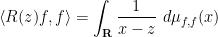
We can depolarise these measures by defining

\displaystyle \mu_{f,g} := \frac{1}{4}( \mu_{f+g,f+g} - \mu_{f-g,f-g} + i \mu_{f+ig,f+ig} - i \mu_{f-ig,f-ig} )

to obtain complex measures
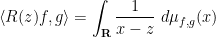
 {\mu_{f,g}} for any {f,g \in H} such that

\displaystyle \langle R(z) f, g \rangle = \int_{\bf R} \frac{1}{x-z}\ d\mu_{f,g}(x)

for all {z} in either the upper or lower half-plane. From duality we see that this uniquely defines {\mu_{f,g}}. In particular, {\mu_{f,g}} depends sesquilinearly on {f,g}, and {\mu_{g,f} = \overline{\mu_{f,g}}}. Also, since each {\mu_{f,f}} has mass {\|f\|^2}, we see that the inner product {\langle f, g\rangle} can be recovered from the spectral measure {\mu_{f,g}}:

\displaystyle \langle f, g \rangle = \int_{\bf R} \ d\mu_{f,g}(x). \ \ \ \ \ (10)


Exercise 16 With the above notation and assumptions, establish the bound {\|\mu_{f,g} \|_{TV} \ll \|f\| \|g\|} for all {f,g \in H}. In particular, for any bounded Borel-measurable function {m: {\bf R} \rightarrow {\bf C}}, there exists a unique bounded operator
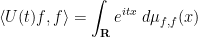
 {m(L): H \rightarrow H} such that

\displaystyle \langle m(L) f, g \rangle = \int_{\bf R} m(x)\ d\mu_{f,g}(x). \ \ \ \ \ (11)


Thus, for instance {m(L)} is the identity when {m=1}, and {m(L) = R(z)} when {m(x) = \frac{1}{x-z}}.

We have just created a map {m \mapsto m(L)} from the bounded Borel-measurable functions {B({\bf R} \rightarrow {\bf C})} on {{\bf R}}, to the bounded operators {B(H \rightarrow H)} on {H}. Now we verify some basic properties of this map.

Exercise 17 (Bounded functional calculus) Let {L: D \rightarrow H} be a self-adjoint densely defined operator, and let {m \mapsto m(L)} be as above.

  • (i) Show that the map {m \mapsto m(L)} is {*}-linear. In particular, if {m} is real-valued, then {m(L)} is self-adjoint.
  • (ii) For any {f, g \in H} and any strictly complex {z}, show that {d\mu_{R(z) f, g}(x) = \frac{1}{x-z}\ d\mu_{f,g}(x)}. (Hint: use the resolvent identity.)
  • (iii) For any {f,g \in H} and any {m \in B({\bf R} \rightarrow {\bf C})}, show that {d\mu_{m(L) f, g} = m\ d\mu_{f,g}}.
  • (iv) Show that the map {m \mapsto m(L)} is a {*}-homomorphism. In particular, {m(L)} and {m'(L)} commute for all {m,m'\in B({\bf R} \rightarrow {\bf C})}.
  • (v) Show that {\|m(L)\|_{op} \ll \sup_{x \in {\bf R}} |m(x)|} for all {m \in B({\bf R} \rightarrow {\bf C})}. Improve the {\ll} to {\leq}. (Hint: to get this improvement, use the {TT^*} identity {\|T\|_{op} = \|TT^* \|_{op}^{1/2}} and the tensor power trick.)
  • (vi) For any Borel subset {E} of {{\bf R}}, show that {\mu(E) := 1_E(L)} is an orthogonal projection of {H}. Show that {\mu} is a countably additive projection-valued measure, thus {\sum_{n=1}^\infty \mu(E_n) = \mu(\bigcup_{n=1}^\infty E_n)} for any sequence of disjoint Borel {E_n}, where the convergence is in the strong operator topology.
  • (vii) For any bounded Borel set {E}, show that the image of {\mu(E)} lies in {D}.
  • (viii) Show that for any {f \in D} and {g \in H}, one has {d\mu_{Lf,g}(x) = x\ d\mu_{f,g}(x)}.
  • (ix) Let {D_c} be the union of the images of {\mu([-N,N])} for {N=1,2,\ldots}. Show that {D_c} is a dense subspace of {D} (and hence of {H}), and that {L} maps {D_c} to {D_c}.
  • (x) Show that {D} is the space of all functions {f \in H} such that {\int_{\bf R} |x|^2\ d\mu_{f,f}(x) < \infty}. Conclude in particular that {m(L)} maps {D} to {D} for all {m \in B({\bf R} \rightarrow {\bf C})}.
  • (xi) If {m, m' \in B({\bf R} \rightarrow {\bf C})} is such that {m'(x) = x m(x)} for all {x \in {\bf R}}, show that {m(L)} takes values in {D}, that {m'(L) f= L m(L) f} for all {f \in H}, and {m'(L) f = m(L) L f} for all {f \in D}.
  • (xii) Let {\sigma(L)} be the space of all {z} such that {L-z: D \rightarrow H} is not invertible. Show that {\sigma(L)} is a closed set which is the union of the supports of the {\mu_{f,g}} as {f,g} range over {H}. In particular, {\sigma(L) \subset {\bf R}}, and {\sigma(L) \subset [0,+\infty)} when {L} is positive. Show that {\mu(\sigma(L)) = \mu({\bf R})} is the identity map.
  • (xiii) Extend the bounded functional calculus from the bounded Borel measurable functions {B({\bf R}\rightarrow{\bf C})} on {{\bf R}} to the bounded measurable functions {B(\sigma(L)\rightarrow{\bf C})} on the spectrum {\sigma(L)} (i.e. show that the previous statements (i)-(xi) continue to hold after {{\bf R}} is replaced by {\sigma(L)} throughout).

The above collection of facts (or various subcollections thereof) is often referred to as the spectral theorem. It is stated for self-adjoint operators, but one can of course generalise the spectral theorem to essentially self-adjoint operators by applying the spectral theorem to the closure. (One has to replace the domain {D} of {L} by the domain {\overline{D}} of the closure {\overline{L}}, of course, when doing so.)

Exercise 18 (Spectral measure and eigenfunctions) Let the notation be as in the preceding exercise, and let {\lambda \in {\bf R}}. Show that the space {\{ f \in D: Lf = \lambda f \}} is the range of the projection {\mu(\{\lambda\})}. In particular, {L} has an eigenfunction at {\lambda} if and only if {\mu(\{\lambda\})} is non-trivial.

We have seen how the existence of resolvents gives us a bounded functional calculus (i.e. the conclusions in the above exercise). Conversely, if a symmetric densely defined closed operator {L} has a bounded functional calculus, one can define the resolvents {R(z)} simply as {m_z(L)}, where {m_z(x) := \frac{1}{x-z}}. Thus we see that the existence of a bounded functional calculus is equivalent to the existence of resolvents, which by the previous discussion is equivalent to self-adjointness.

Using the bounded functional calculus, one can not only recover the resolvents {R(z)}, but can now also build Schrödinger propagators {e^{itL}}, and when {L} is positive definite one can also build heat operators {e^{tL}} for {t > 0} and wave operators {e^{it\sqrt{L}}} for {t \in {\bf R}} (and also define resolvents {R(-k^2)} for negative choices {-k^2} of the spectral parameter). We will study these operators more in the next section.

Exercise 19 (Locally bounded functional calculus) Let {L: D \rightarrow H} be a densely defined self-adjoint operator, and let {B_{loc}(\sigma(L) \rightarrow {\bf C})} be the space of Borel-measurable functions from {\sigma(L)} to {{\bf C}} which are bounded on every bounded set.

  • Show that for every {m \in B_{loc}(\sigma(L) \rightarrow {\bf C})} there is a unique linear operator {m(L): D_c \rightarrow D_c} such that

    \displaystyle d\mu_{m(L)f,g}(x) = m(x)\ d\mu_{f,g}(x)

    whenever {f,g \in D_c}.

  • (i) Show that the map {m \mapsto m(L)} is a {*}-homomorphism.
  • (ii) Show that when {m} is actually bounded (rather than merely locally bounded), then this definition of {m(L)} agrees with that in the preceding exercise (after restricting from {H} to {D_c}).
  • (iii) Show that {L = \iota(L)}, where {\iota} is the identity map {\iota(x) := x}.
  • (iv) State and prove a rigorous version of the formal assertion that

    \displaystyle L = \int_{\bf R} xd \mu(x)

    and more generally

    \displaystyle m(L) = \int_{\bf R} m(x) d \mu(x).

Now we use the spectral theorem to place self-adjoint operators in a normal form. Let us say that two operators {L: D \rightarrow H} and {L': D' \rightarrow H'} are unitarily equivalent if there is a unitary map {U: H \rightarrow H'} with {U(D)=D'} and {L' = U^{-1} L U}. It is easy to see that all the constructions given above (such as the bounded functional calculus) are preserved by unitary equivalence.

If {L: D \rightarrow H} is a densely defined self-adjoint operator, define an invariant subspace to be a subspace {V} of {H} such that {m(L) V \subset V} for all {m \in B(\sigma(L) \rightarrow {\bf C})}. We say that a vector {f \in H} is a cyclic vector for {H} if the set {\{ m(L) f: m \in B(\sigma(L) \rightarrow {\bf C})\}} is dense in {H}.

Exercise 20

  • (i) Show that if {V} is an invariant subspace of {H}, then so is {V^\perp}, and furthermore the orthogonal projections to {V} and {V^\perp} commute with {m(L)} for every {m \in B(\sigma(L) \rightarrow {\bf C})}.
  • (ii) Show that if {V} is a invariant subspace of {H}, then the restriction {L\downharpoonright_V: D \cap V \rightarrow V} of {L} to {V} is a densely defined self-adjoint operator on {V} with {\sigma(L\downharpoonright_V) \subset\sigma(L)}. Furthermore, one has {m(L\downharpoonright_V) = m(L)\downharpoonright_V} for all {m \in B(\sigma(L) \rightarrow {\bf C})}.
  • (iii) Show that {H} decomposes as a direct sum {\bigoplus_{\alpha \in A} H_\alpha}, where the index set {A} is at most countable, and each {H_\alpha} is a closed invariant subspace of {H} (with the {H_\alpha} mutually orthogonal), such that each {H_\alpha} has a cyclic vector {f_\alpha}. (Hint: use Zorn’s lemma and the separability of {H}.)
  • (iv) If {H} has a cyclic vector {f_0}, show that {L} is unitarily conjugate to a multiplication operator {f(x) \mapsto x f(x)} on {L^2({\bf R},\nu)} for some non-negative Radon measure {\nu}, defined on the domain {\{ f \in L^2({\bf R},\nu): xf \in L^2({\bf R},\nu) \}}.
  • (v) For general {H}, show that {L} is unitarily conjugate to a multiplication operator {f(x) \mapsto g(x) f(x)} on {L^2(X,\nu)} for some measure space {(X,\nu)} with a countably generated {\sigma}-algebra and some measurable {g: X \rightarrow {\bf R}}, defined on the domain {\{ f \in L^2(X,\nu): gf \in L^2(X,\nu) \}}.

The above exercise gives a satisfactory concrete description of a self-adjoint operator (up to unitary equivalence) as a multiplication operator on some measure space {L^2(X,\nu)}, although we caution that this equivalence is not canonical (there is some flexibility in the choice of the underlying measure space {(X,\nu)} and multiplier {g}, as well as the unitary conjugation map).

Exercise 21 Let {L: D \rightarrow H} be a self-adjoint densely defined operator.

  • (i) Show that {L} is positive if and only if {\sigma(L) \subset [0,+\infty)}.
  • (ii) Show that {L} is bounded if and only if {\sigma(L)} is bounded. Furthermore, in this case we have {\|L\|_{op} = \sup_{x \in \sigma(L)} |x|}.
  • (iii) Show that {H} is trivial if and only if {\sigma(L)} is empty.

— 3. Self-adjointness and flows —

Now we relate self-adjointness to a variety of flows, beginning with the heat flow.

Exercise 22 Let {L: D \rightarrow H} be a self-adjoint positive densely defined operator, and for each {t \geq 0}, let {S(t): H \rightarrow H} be the heat operator {S(t) := e^{-tL}}.

  • (i) Show that for each {t \geq 0}, {S(t)} is a bounded self-adjoint operator of norm at most {1}, that the map {t \mapsto S(t)} is continuous in the strong operator topology, and such that {S(0)=1} and {S(t)S(t') = S(t+t')} for all {t,t' \geq 0}. (The latter two properties are asserting that {t \mapsto S(t)} is a one-parameter semigroup.)
  • (ii) Show that for any {f \in D}, {\frac{S(t) f - f}{t}} converges to {-Lf} as {t \rightarrow 0^+}.
  • (iii) Conversely, if {f \in H} is not in {D}, show that {\frac{S(t) f - f}{t}} does not converge as {t \rightarrow 0^+}.

We remark that the above exercise can be viewed as a special case of the Hille-Yoshida theorem.

We now establish a converse to the above statement:

Theorem 5 Let {H} be a separable Hilbert space, and suppose one has a family {t \mapsto S(t)} of bounded self-adjoint operators of norm at most {1} for each {t \geq 0}, which is continuous in the strong operator topology, and such that {S(0)=1} and {S(t) S(t') = S(t+t')} for all {t,t' \geq 0}. Then there exists a unique self-adjoint positive densely defined operator {L: D \rightarrow H} such that {S(t) = e^{-tL}} for all {t \geq 0}.

We leave the proof of this result to the exercise below. The basic idea is to somehow use the identity

\displaystyle (x+1)^{-1} = \int_0^\infty e^{-tx} e^{-t}\ dt

which suggests that

\displaystyle (L+1)^{-1} = \int_0^\infty S(t) e^{-t}\ dt

which should allow one to recover {L} from the {S(t)}.

Exercise 23 Let the notation be as in the above theorem.

  • (i) Establish the uniqueness claim. (Hint: use Exercise 22.)
  • (ii) Let {R} be the operator

    \displaystyle R := \int_0^\infty S(t) e^{-t}\ dt.

    Show that {R} is well-defined, bounded, positive semidefinite, and self-adjoint, with operator norm at most one, and that {R} commutes with all the {S(t)}.

  • (iii) Show that the spectrum of {R} lies in {[0,1]}, but that {R} has no eigenvalue at {0}.
  • (iv) Show that there exists a densely defined self-adjoint operator {R^{-1}: D \rightarrow H} such that {RR^{-1}} is the identity on {D} and {R^{-1} R} is the identity on {H}.
  • (v) Show that {L := R^{-1}-1} is densely defined self-adjoint and positive definite, and commutes with all the {S(t)}.
  • (vi) Show that for all {v \in H} and {t \geq 0}, one has {\frac{d}{dt} S(t) Rf = -L S(t) Rf} and {\frac{d}{dt} e^{-tL} Rf = - L e^{-tL} Rf}, where the derivatives are in the classical limiting Newton quotient sense (in the strong topology of {H}).
  • (vii) Conclude the proof of Theorem 5. (Hint: show that {\frac{d}{dt} \|S(t)Rf - e^{-tL} Rf\|^2} is non-positive.)

The above exercise gives an important way to establish essential self-adjointness, namely by solving the heat equation (1):

Exercise 24 Let {L: D \rightarrow H} be a densely defined symmetric positive definite operator. Suppose that for every {f \in D} there exists a continuously differentiable solution {u: [0,+\infty) \rightarrow D} to (1). Show that {L} is essentially self-adjoint. (Hint: by investigating {\frac{d}{dt} \| u(t)\|^2}, establish the uniqueness of solutions to the heat equation, which allows one to define linear contractions {S(t)}. To establish self-adjointness of the {S(t)}, take an inner product of a solution to the heat equation against a time-reversed solution to the heat equation, and differentiate that inner product in time. Now apply the preceding exercises to obtain a self-adjoint extension {L': D' \rightarrow H} of {L}. To show that {L'} is the closure of {L}, it suffices to show that {D} is dense in {D'} with the inner product {\langle f, g \rangle + \langle L' f, g \rangle}. But if {D} is not dense in {D'}, then it has a non-trivial orthogonal complement; apply {S(t)} to this complement to show that {D} also has a non-trivial orthogonal complement in {H}, a contradiction.)

Remark 2 When applying the above criterion for essential self-adjointness, one usually cannot use the space {C^\infty_c} of compactly supported smooth functions as the dense subspace, because this space is usually not preserved by the heat flow. However, in practice one can get around this by enlarging the class, for instance to the class of Schwartz functions.

Now we obtain analogous results for the Schrödinger propagators {e^{itL}}. We begin with the analogue of Exercise 22:

Exercise 25 Let {L: D \rightarrow H} be a self-adjoint densely defined operator, and for each {t \in {\bf R}}, let {U(t): H \rightarrow H} be the Schrödinger operator {S(t) := e^{itL}}.

  • (i) Show that for each {t \in {\bf R}}, {U(t)} is a unitary operator, that the map {t \mapsto U(t)} is continuous in the strong operator topology, and such that {U(0)=1} and {U(t)U(t') = U(t+t')} for all {t,t' \geq 0}.
  • (ii) Show that for any {f \in D}, {\frac{U(t) f - f}{t}} converges to {iLf} as {t \rightarrow 0}.
  • (iii) Conversely, if {f \in H} is not in {D}, show that {\frac{U(t) f - f}{t}} does not converge as {t \rightarrow 0}.

Now we can give the converse, known as Stone’s theorem on one-parameter unitary groups:

Theorem 6 (Stone’s theorem) Let {H} be a separable Hilbert space, and suppose one has a family {t \mapsto U(t)} of unitary for each {t \in {\bf R}}, which is continuous in the strong operator topology, and such that {U(0)=1} and {U(t) U(t') = U(t+t')} for all {t,t' \in {\bf R}}. Then there exists a unique self-adjoint densely defined operator {L: D \rightarrow H} such that {U(t) = e^{itL}} for all {t \in {\bf R}}.

We outline a proof of this theorem in an exercise below, based on using the group {U(t)} to build spectral measure.

Exercise 26 Let the notation be as in the above theorem.

  • (i) Establish the uniqueness component of Stone’s theorem.
  • (ii) Show that for any {f \in H}, there is a non-negative Radon measure {\mu_{f,f}} of total mass {\|f\|^2} such that

    \displaystyle \langle U(t) f, f \rangle = \int_{\bf R} e^{itx}\ d\mu_{f,f}(x)

    for all {t \in {\bf R}}. (Hint: use Bochner’s theorem, a proof of which (at least on {{\bf R}}, which is the case of interest here) can be found for instance in these notes.)

  • (iii) Show that for any {f,g \in H}, there is a unique complex measure {\mu_{f,g}} such that

    \displaystyle \langle U(t) f, g \rangle = \int_{\bf R} e^{itx}\ d\mu_{f,g}(x)

    for all {t \in {\bf R}}. Show that {\mu_{f,g}} is sesquilinear in {f,g} with {\mu_{g,f} = \overline{\mu_{f,g}}}.

  • (iv) Show that for any {m \in B({\bf R} \rightarrow {\bf C})}, there is a unique bounded operator {m(L): H \rightarrow H} such that

    \displaystyle \langle m(L) f, g \rangle = \int_{\bf R} m(x)\ d\mu_{f,g}(x)

    for all {f,g \in H}.

  • (v) Show that {d\mu_{m(L)f,g}(x) = m(x)\ d\mu_{f,g}(x)} for all {m \in B({\bf R} \rightarrow {\bf C})} and {f,g \in H}.
  • (vi) Show that the map {m \mapsto m(L)} is a *-homomorphism from {B({\bf R} \rightarrow {\bf C})} to {B(H \rightarrow H)}.
  • (vii) Show that there is a projection-valued measure {\mu} with {\mu({\bf R}) = 1}, such that for every {f, g}, the complex measure {\mu_{f,g} := \langle \mu f, g \rangle} is such that

    \displaystyle \langle U(t) f, g \rangle = \int_{\bf R} e^{itx}\ d\mu_{f,g}(x)

    for all {t \in {\bf R}}.

  • (viii) Show that there exists a self-adjoint densely defined operator {L: D \rightarrow H} whose spectral measure is {\mu}.
  • (ix) Conclude the proof of Stone’s theorem.

Exercise 27 Let {L: D \rightarrow H} be a densely defined symmetric operator. Suppose that for every {f \in D} there exists a continuously differentiable solution {u: {\bf R}\rightarrow D} to (2). Show that {L} is essentially self-adjoint.

We can now see a clear link between essential self-adjointness and completeness, at least in the case of scalar first-order differential operators:

Exercise 28 Let {M} be a smooth manifold with a smooth measure {\mu}, and let {X} be a smooth vector field on {M} which is divergence-free with respect to the measure {\mu}. Suppose that the vector field {X} is complete in the sense that for any {x_0 \in M}, there exists a global smooth solution {x: {\bf R} \rightarrow M} to the ODE {\frac{d}{dt} x(t) = X(x(t))} with initial data {x(0)=x_0}. Show that the first-order differential operator {i \nabla_X: C_c(M) \rightarrow L^2(M)} is essentially self-adjoint.

Extend the above result to non-divergence-free vector fields, after replacing {\nabla_X} with {\nabla_X + \frac{1}{2} \hbox{div}(X)}.

Remark 3 The requirement of completeness is basically necessary; one can still have essential self-adjointness if there are a measure zero set of initial data {x_0} for which the trajectories of {X} are incomplete, but once a positive measure set of trajectories become incomplete, the propagators {\exp( t \nabla_X )} do not make sense globally, and so self-adjointness should fail.

Finally, we turn to the relationship between self-adjointness and the wave equation, which is a more complicated variant of the relationship between self-adjointness and the Schrödinger equation. More precisely, we will show the following version of Exercise 27:

Theorem 7 Let {L: D \rightarrow H} be a densely defined positive symmetric operator. Suppose for every {f, g \in D}, there exists a twice continuously differentiable (in {D}) solution {u: {\bf R} \rightarrow D} to (3). Then {L} is essentially self-adjoint.

(One could also obtain wave equation analogues of Exercise 25 or Theorem 6, but these are somewhat messy to state, and we will not do so here.)

We now prove this theorem. To simplify the exposition, we will assume that {L} is strictly positive, in the sense that {\langle Lf, f \rangle > 0} for all non-zero {f \in D}, and leave the general case as an exercise.

We introduce a new inner product {\langle, \rangle_{\dot H^1}} on {D} by the formula

\displaystyle \langle f, g \rangle_{\dot H^1} := \langle Lf, g \rangle.

By hypothesis, this is a Hermitian inner product on {D}. We then define an inner product {\langle, \rangle_E} on {D \times D} by the formula

\displaystyle \langle (u_0,u_1), (v_0,v_1) \rangle_E := \langle u_0, v_0 \rangle_{\dot H^1} + \langle u_1, v_1 \rangle,

then this is a Hermitian inner product on {D \times D}. We define the energy space {{\mathcal E}} be the completion of {D \times D} with respect to this inner product; we can factor this as {{\mathcal E} = \dot H^1 \times H}, where {\dot H^1} is the completion of {D} using the {\dot H^1} inner product.

Suppose {u: {\bf R} \rightarrow D} is a twice continuously differentiable solution to (3) for some {f,g \in D}. Then if we define the energy

\displaystyle E(t) := \frac{1}{2} \langle (u, \partial t u),(u, \partial t u) \rangle_E,

then one easily computes using (3) that {\partial_t E(t) = 0}, and so

\displaystyle E(t) = E(0) = \frac{1}{2} \langle (f, g), (f,g) \rangle_E.

In particular, if {f=g=0}, then {u=0}, and so twice continuously differentiable solutions to (3) are unique. This allows us to define wave operators {W(t): D \times D \rightarrow D \times D} by defining {W(t)(f,g) := (u(t), \partial_t u(t))}. This is clearly linear, and from the energy identity we see that {W} is an isometry, and thus extends to an isometry on the energy space {{\mathcal E}}. From uniqueness we also see that {t \mapsto W(t)} is a one-parameter group, i.e. a homomorphism that is continuous in the strong operator topology. In particular, the isometries {W(t)} are invertible and are thus unitary. By Stone’s theorem, there thus exists a densely defined self-adjoint operator {A: \tilde D \rightarrow {\mathcal E}} on some dense subspace {\tilde D} of {{\mathcal E}} such that {W(t) = e^{itA}} for all {t \in {\bf R}}.

If {(f,g) \in D \times D}, then from the twice differentiability of the solution {u} to the wave equation, we see that

\displaystyle \lim_{t \rightarrow 0} \frac{W(t)(f,g) - (f,g)}{t} = (g, -L f).

From Exercise 2, we conclude that {D \times D \subset \tilde D} and

\displaystyle A(f,g) = (-ig,iL f) \ \ \ \ \ (12)


for all {(f,g) \in D \times D}.

Now we need to pass from the self-adjointness of {A} to the essential self-adjointness of {L}. Suppose for contradiction that {L} was not essentially self-adjoint. Then {L+1} does not have dense image, and so there exists a non-zero {h \in H} such that

\displaystyle \langle (L+1) f, h \rangle = 0

for all {f \in D}.

It will be convenient to work with a “band-limited” portion of {D \times D}, to get around the problem that {A} and {L} can leave this domain. Let {\phi: {\bf R} \rightarrow {\bf R}} be a compactly supported even smooth function of total mass one. For any {R>0}, define the Littlewood-Paley projection

\displaystyle P_{\leq R} := \int_{\bf R} R \phi(R t) W(t)\ dt = \int_{\bf R} R \phi(Rt) e^{itA}\ dt = \hat \phi( A/R ),

where {\hat \phi} is the Schwartz function {\hat \phi(\xi) := \int_{\bf R} \phi(t) e^{it\xi}\ dt}. Then (by strong continuity of {W(t)}) these operators map {D\times D} to {D \times D}, commutes with the entire functional calculus of {A}, and also maps {{\mathcal E}} to {\tilde D}. Also, from functional calculus one sees that

\displaystyle A P_{\leq R} = i \int_{\bf R} R^2 \phi'(Rt) W(t)\ dt

and in particular {A P_{\leq R}} maps {D \times D} to {D \times D} as well.

Let {\tau: {\mathcal E} \rightarrow {\mathcal E}} be the reflection operator {\tau(f,g) := (f,-g)}. From time reversal of the wave equation, we have {W(t) \tau = \tau W(-t)}, and thus {\tau} commutes with {P_{\leq R}}. In particular, we can write

\displaystyle P_{\leq R} (f,g) = (P_{\leq R}^0 f, P_{\leq R}^1 g)

for some operators {P_{\leq R}^0: \dot H^1 \rightarrow \dot H^1} and {P_{\leq R}^1: H \rightarrow H}. Since {P_{\leq R}} preserves {D \times D}, the operators {P_{\leq R}^0, P_{\leq R}^1} preserve {D}.

For any {(f,g) \in D \times D}, we have

\displaystyle P_{\leq R} A(f,g) = A P_{\leq R}(f,g);

combining this with (12) we see that

\displaystyle P_{\leq R}^0 g = P_{\leq R}^1 g

and

\displaystyle P_{\leq R}^1 Lf = L P_{\leq R}^0 f

for all {f, g \in D}. Also, since {A P_{\leq R}} preserves {D \times D}, we see that {L P_{\leq R}^0 = P_{\leq R}^1 L} preserves {D}.

We can then expand {A^2 P_{\leq R}(f,g)} as

\displaystyle A P_{\leq R} A (f,g) = A P_{\leq R} (-ig, iLf )

\displaystyle = A (-i P_{\leq R}^1 g, i L P_{\leq R}^0 f )

\displaystyle = (L P_{\leq R}^0 f, L P_{\leq R}^1 g)

and thus

\displaystyle (A^2+1) P_{\leq R}(f,g) = ((L+1) P_{\leq R}^0 f, (L+1) P_{\leq R}^1 g).

In particular

\displaystyle \langle (A^2+1) P_{\leq R}(f,g), (0,h) \rangle_{\mathcal E} = 0

for all {(f,g) \in D \times D}. By duality (noting that {(A^2+1) P_{\leq R}} is a bounded real function of {A}) we conclude that

\displaystyle (A^2+1) P_{\leq R} (0,h) = 0

But by sending {R \rightarrow \infty} and using the spectral theorem, this implies from monotone convergence that the spectral measure {\mu_{(0,h),(0,h)}} is zero, and thus {(0,h)} vanishes in {{\mathcal E}}, a contradiction. This establishes the essential self-adjointness of {L}.

Exercise 29 Establish Theorem 7 without the assumption that {L} is strictly positive. (Hint: use the Cauchy-Schwarz inequality to show that strict positivity is equivalent to the absence of eigenfunctions with eigenvalue zero, and then quotient out such eigenfunctions.)

— 4. Essential self-adjointness of the Laplace-Beltrami operator —

We now discuss how one can use the above criteria to establish essential self-adjointness of a Laplace-Beltrami operator {-\Delta_g} on a smooth complete Riemannian manifold {(M,g)}, viewed as a densely defined symmetric positive operator on the dense subspace {C^\infty_c(M)} of {L^2(M)}. This result was first established by Gaffney and by Roelcke.

To do this, we have to solve a PDE – either the Helmholtz equation (4) (for some {z} not on the positive real axis), the heat equation (1), the Schrödinger equation (25), or the wave equation (3).

The Schrödinger formalism is quite suggestive. From a semiclassical perspective, the Schrödinger equation associated to the Laplace-Beltrami operator {-\Delta_g} should be viewed as a quantum version of the classical flow associated to the corresponding Hamiltonian {g^{ij}(x) \xi_i \xi_j}, i.e. geodesic flow. From Exercise 28 we know that the generator of Hamiltonian flows (normalised by {i}) are essentially self-adjoint when they are complete (note from Liouville’s theorem that such generators are automatically divergence-free with respect to Liouville measure), which suggests that the Schrödinger operator {-\Delta_g} should be also. Unfortunately, this is not a rigorous argument, and is difficult to make it so due to the nature of the time-dependent Schrödinger equation, which has infinite speed of propagation, and no dissipative properties. In practice, we therefore establish esssential self-adjointness by solving one of the other equations.

To solve any of these equations, it is difficult to solve any of them by an exact formula (unless the manifold {M} is extremely symmetric); but one can proceed by solving them approximately, and using perturbation theory to eliminate the error. This method works as long as the error created by the approximate solution is both sufficiently small and sufficiently smooth that perturbative techniques (such as Neumann series, or the inverse function theorem) become applicable. (This type of method, for instance, is used to deduce essential self-adjointness of various perturbations {-\Delta+V} of the Laplace-Beltrami operator from the essential self-adjointness of the original operator {-\Delta}.)

For instance, suppose one is trying to solve the Helmholtz equation

\displaystyle (-\Delta_g + k^2) u = f

for some large real {k}, and some {f \in L^2(M)}. For sake of concreteness let us take {M} to be three-dimensional. If {M} was a Euclidean space {{\bf R}^3}, then we have an explicit formula

\displaystyle u(x) = \frac{1}{4\pi} \int_{{\bf R}^3} \frac{e^{-k|x-y|}}{|x-y|} f(y)\ dy

for the solution; note that the exponential decay of {e^{-k|x-y|}} will keep {u} in {L^2} as well. Inspired by this, we can try to solve the Helmholtz equation in curved space by proposing as an approximate solution

\displaystyle u(x) = \frac{1}{4\pi} \int_{M} \frac{e^{-k d(x,y)}}{d(x,y)} f(y)\ dg(y).

This is a little problematic because {d(x,y)} develops singularities after a certain point, but if one has a uniform lower bound on the injectivity radius (here we are implicitly using the hypothesis of completeness), and also uniform bounds on the curvature and its derivatives, one can truncate this approximate solution to the region where {d(x,y)} is small, and obtain an approximate solution {u} whose error

\displaystyle e := (-\Delta_g + k^2) u - f

can be made to be smaller in {L^2} norm than that of {f} if the spectral parameter {k} is chosen large enough; we omit the details. From this, we can then solve the Helmholtz equation by Neumann series and thus establish essential self-adjointness. A similar method also works (under the same hypotheses on {M}) to construct approximate heat kernels, giving another way to establish essential self-adjointness of the Laplace-Beltrami operator.

What about when there is no uniform bound on the geometry? In that case, it is best to work with the wave equation formalism, because the finite speed of propagation property of that equation allows one to localise to compact portions of the manifold for which uniform bounds on the geometry are automatic. Indeed, to solve the wave equation in {C^\infty_c(M)} for some fixed period of time, one can use finite speed of propagation, combined with completeness of the manifold, to work in a compact subset of this manifold, which by suitable alteration of the metric beyond the support of the solution, one can view as a subset of a compact complete manifold. On such manifolds, we already know essential self-adjointness by the previous arguments, so we may solve the wave equation in that setting (one can also solve the wave equation using methods from microlocal analysis, if desired), and then take repeated advantage of finite speed of propagation (which can be proven rigorously by energy methods) to glue together these local solutions to obtain a global solution; we omit the details.

In all these cases, a somewhat nontrivial application of PDE theory is required. Unfortunately, this seems to be inevitable; at some point one must somehow use the hypothesis of completeness of the underlying manifold, and PDE methods are the only known way to connect that hypothesis to the dynamics of the Laplace-Beltrami operator.