Let  be
be  Hermitian matrices, with eigenvalues
  and
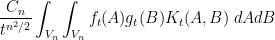
and  . The Harish-Chandra–Itzykson-Zuber integral formula exactly computes the integral
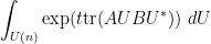
where  is integrated over the Haar probability measure of the unitary group
  and
and  is a non-zero complex parameter, as the expression
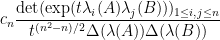
when the eigenvalues of  are simple, where
  denotes the Vandermonde determinant

and  is the constant

There are at least two standard ways to prove this formula in the literature. One way is by applying the Duistermaat-Heckman theorem to the pushforward of Liouville measure on the coadjoint orbit  (or more precisely, a rotation of such an orbit by
  ) under the moment map
  , and then using a stationary phase expansion. Another way, which I only learned about recently, is to use the formulae for evolution of eigenvalues under Dyson Brownian motion (as well as the closely related formulae for the GUE ensemble), which were derived in this previous blog post. Both of these approaches can be found in several places in the literature (the former being observed in the original paper of Duistermaat and Heckman, and the latter observed in the paper of Itzykson and Zuber as well as in this later paper of Johansson), but I thought I would record both of these here for my own benefit.
The Harish-Chandra-Itzykson-Zuber formula can be extended to other compact Lie groups than . At first glance, this might suggest that these formulae could be of use in the study of the GOE ensemble, but unfortunately the Lie algebra associated to  corresponds to real anti-symmetric matrices rather than real symmetric matrices. This also occurs in the case, but there one can simply multiply by to rotate a complex skew-Hermitian matrix into a complex Hermitian matrix. This is consistent, though, with the fact that the (somewhat rarely studied) anti-symmetric GOE ensemble has cleaner formulae (in particular, having a determinantal structure similar to GUE) than the (much more commonly studied) symmetric GOE ensemble.
— 1. Dyson Brownian motion argument —
Let  denote the space of Hermitian matrices. We place a Haar measure
  on this space; the exact normalisation of this measure will ultimately not be relevant (it will create a number of factors which will eventually cancel each other out). Define an invariant function on to be a function
  which is invariant with respect to conjugations, thus
 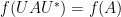 for all
  and
and  . Thus the value
  of an invariant function at a Hermitian matrix depends only on the eigenvalues , and so by abuse of notation we may write

where  is now a function on the Weyl chamber

By the Riesz representation theorem, there must be some density function  with the property that
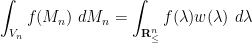
where  is Lebesgue measure on
  , and
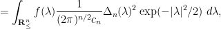
, and  is an invariant function with sufficient regularity and decay (e.g. smooth and exponentially decaying will certainly suffice). To compute this density function, we can exploit the explicit formulae for the GUE ensemble. As discussed in this previous blog post, the GUE ensemble is a probability measure on with probability density

for some normalisation constant  (the exact choice of which depends on how one normalised ), and the eigenvalues of GUE have the probability density

Computing the expectation of  for a GUE matrix
  using these formulae for an invariant function with sufficient regularity and decay, we conclude that

and hence (since 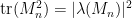 )
)

and so

for any invariant function with sufficient regularity and decay.
Now let  be two invariant functions with sufficient regularity and decay to justify all the computations that follow, let be a positive real number, and consider the integral

which is the bilinear form associated to the heat flow on for time . We will evaluate this integral in two different ways. On the one hand, we can expand the integral as

where  and
and  . Next, conjugating
  by an arbitrary unitary matrix and then integrating over Haar measure on , we can rewrite this as
where

The expression  invariant in both
  and , so by two applications of (1) we can thus write (2) as

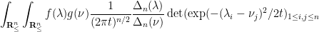
Now we compute (2) another way. For fixed , the integral

can be interpreted as the expectation of  where
where  is a copy of GUE. By the Brezin-Hikami-Johansson formula (see Theorem 7 of these notes), the eigenvalues of
  are distributed according to the density

and so the previous integral can be written as

(Note: in the paper of Johansson, two proofs of the Brezin-Hikami-Johansson formula were given; one via the Harish-Chandra-Itzykson-Zuber formula discussed in this post, and the other via solving the equations of Dyson Brownian motion. The former proof of course cannot be invoked here as it would be circular, but the latter proof, which is the one used in the notes linked to above, can be used without risk of circularity.)
Integrating the above formula against  and then using (1), we may thus write (2) as

Comparing this against (3), we conclude that

and so

This equation was derived for all positive real , but by analytic continuation it is then true for all non-zero complex . Replacing by  we obtain the Harish-Chandra-Itzykson-Zuber integral formula.
— 2. The Duistermaat-Heckman theorem —
The Duistermaat-Heckman theorem concerns a significantly more general situation than the one appearing in the Harish-Chandra-Itzykson-Zuber integral formula, namely that of a symplectic manifold with a torus action that is associated to a moment map. To describe this theorem, it is simplest to begin with the one-dimensional setting of Hamiltonian circle actions on a symplectic manifold. (I will assume here some familiarity with differential forms on smooth manifolds, and also freely use infinitesimals in place of more traditional calculus notation at times.)
Recall that a symplectic manifold  is a smooth manifold
  equipped with a symplectic form
  , that is to say a smooth anti-symmetric two-form
  on which is both non-degenerate (thus
  whenever
  is a vector field that is non-vanishing at
  ) and closed (thus
  ). Symplectic manifolds are necessarily even dimensional (because odd-dimensional anti-symmetric real matrices automatically have a zero eigenvalue and are thus degenerate). If
  is a
is a  -dimensional manifold, the Liouville measure on that manifold is defined as the volume form
  , where we use
  to denote the
  -fold wedge product of with itself, and (by abuse of notation) we identify volume forms with measures. (Note that wedge product is a commutative operation on even-order forms such as .)
Given a smooth function  on a symplectic manifold (called the Hamiltonian), one can associate the Hamiltonian vector field
  , defined by requiring that

or in other words that

for all smooth vector fields  . From the non-degeneracy of , we see that vanishes precisely at the critical (or stationary) points of the Hamiltonian
  .
.
From the Cartan formula

for the Lie derivative of a form along a vector field , we see in the case of the symplectic form and Hamiltonian vector field that

and so the symplectic form is preserved by the vector field . From the product rule we conclude that Liouville measure is also preserved, a fact known as Liouville’s theorem in Hamiltonian mechanics:

We can exponentiate the Hamiltonian vector field to obtain a one-parameter group  of smooth maps for
  :
:

This is a smooth action of the additive group  , and by the preceding discussion, these maps are symplectomorphisms and in particular preserve Liouville measure, thus one can think of
  as a homomorphism from to the symplectomorphism group
  of .
of .
Now suppose that is compact, so that the Liouville measure is finite. We can then pushforward Liouville measure  by the Hamiltonian to create a measure
  on , which we will call the Duistermaat-Heckman measure associated to this Hamiltonian. At present, the Hamiltonian can be an arbitrary smooth function, and so the Duistermaat-Heckman measure is also more or less completely arbitrary. However, we do at least have Sard’s theorem, which asserts that almost every (in the sense of Lebesgue measure) point
  in is a regular value for in the sense that it is not the image
  of a critical point of . In the neighbourhood of each regular point, an application of the inverse function theorem shows that the Duistermaat-Heckman measure is smooth (or more precisely, a smooth multple of Lebesgue.
However, if we make the additional assumption that the Hamiltonian action is periodic (thus it is an action of  and not just of for some period
  ), we can say much more about the Duistermaat-Heckman measure at regular points:
Proposition 1 (Duistermaat-Heckman theorem for circle actions) Let be a -dimensional compact symplectic manifold for some  , and let be a Hamiltonian associated to a periodic action
  of for some period
  . Then, in a sufficiently small neighbourhood of any given regular value of the Duistermaat-Heckman measure is a polynomial multiple of Lebesgue measure, with the polynomial being of degree at most
  .
.
In particular, if has only finitely many critical points, then the Duistermaat-Heckman measure is a piecewise polynomial multiple of Lebesgue measure on .
Let us illustrate this theorem with some key examples. We begin with a near-example, in which the compactness hypothesis is dropped.
Example 1 Let  with the standard symplectic form
  , thus

and Liouville measure is just Lebesgue measure  (using the standard orientation of
  ). Let be the Hamiltonian

for some  and
and  . The only critical point of is at the origin. Then the associated Hamiltonian vector field is
and so (using complex notation  )
)

In particular, the Hamiltonian action is periodic with period  . The Duistermaat-Heckman measure is supported on the half-line
  , with
  being the only non-regular value, and one can compute that it is times Lebesgue measure on this half-line, or equivalently it is the pushforward of Lebesgue measure on
  under the map
  .
.
Example 2 We can make a higher-dimensional (but still non-compact) version of the above example. Let  , and let
  be given the standard symplectic form

so that Liouville measure is again Lebesgue measure. If we let be the Hamiltonian

then the only critical point is at the origin, and the associated Hamiltonian vector field is
and so (using the complex notation  ) we have

We thus see that this flow will also be periodic if the  are commensurate (i.e. linear multiples of each other), and that is the only non-regular value. As for the Duistermaat-Heckman measure, it is the pushforward of Lebesgue measure on the orthant
  by the map
  , which one easily verifies to be a polynomial multiple of Lebesgue measure on , with the polynomial being of degree .
Now we give an example that dates back to Archimedes (two millennia before the formal development of symplectic geometry!).
Example 3 (Archimedes sphere and cylinder) Let  be the unit sphere, which we can coordinatise using the usual spherical coordinates
 ![{\theta \in [0,2\pi]}](https://s0.wp.com/latex.php?latex=%7B%5Ctheta+%5Cin+%5B0%2C2%5Cpi%5D%7D&bg=ffffff&fg=000000&s=0&c=20201002) ,
, ![{\phi \in [0,\pi]}](https://s0.wp.com/latex.php?latex=%7B%5Cphi+%5Cin+%5B0%2C%5Cpi%5D%7D&bg=ffffff&fg=000000&s=0&c=20201002) as
as
![\displaystyle S^2 = \{ (\sin \phi \cos \theta, \sin \phi \sin \theta, \cos \phi): \theta \in [0,2\pi], \phi \in [0,\pi] \}](https://s0.wp.com/latex.php?latex=%5Cdisplaystyle+S%5E2+%3D+%5C%7B+%28%5Csin+%5Cphi+%5Ccos+%5Ctheta%2C+%5Csin+%5Cphi+%5Csin+%5Ctheta%2C+%5Ccos+%5Cphi%29%3A+%5Ctheta+%5Cin+%5B0%2C2%5Cpi%5D%2C+%5Cphi+%5Cin+%5B0%2C%5Cpi%5D+%5C%7D&bg=ffffff&fg=000000&s=0&c=20201002)
with the Riemannian metric

and a symplectic form
and associated Liouville measure  . We take the Hamiltonian
  to be the vertical coordinate function

and the Hamiltonian vector field is then the rotation vector field around the vertical axis:

As such, the exponential map  is the anti-clockwise rotation by radians around the vertical axis:


which is periodic with period  , and the only stationary points are at the north and south poles (so the only non-regular values of are
  and
and  ), and the Duistermaat-Heckman measure is times Lebesgue measure on
 ![{[-1,1]}](https://s0.wp.com/latex.php?latex=%7B%5B-1%2C1%5D%7D&bg=ffffff&fg=000000&s=0&c=20201002) . This latter fact is equivalent to the famous theorem of Archimedes that a sphere and its circumscribing cylinder have the same surface area on horizontal slices.
. This latter fact is equivalent to the famous theorem of Archimedes that a sphere and its circumscribing cylinder have the same surface area on horizontal slices.
Now we prove Proposition 1. Let  be a regular value of . Then, for all sufficiently close to , is also regular, and
  is a
is a  -dimensional manifold on which acts freely, thus one can view as a circle bundle, with the circles being the actions of . By (4), the Hamiltonian vector field, which is tangent to these circles, is symplectically orthogonal to the tangent bundle of . Thus, if we quotient out by the circle action, we obtain a
  -dimensional manifold
  , and the symplectic form restriced to descends to a smooth anti-symmetric form
  on , which is non-degenerate because is non-degenerate. The integral of on any small closed two-dimensional surface lifts up to equal the integral on on a lifted version of that surface; as is closed, we conclude that is also closed. Thus
  is a -dimensional symplectic manifold, known as the symplectic reduction (or Marsden-Weinstein symplectic quotient) of by at the value .
Now consider an infinitesimal -dimensional parallelepiped  in . This can be lifted up (non-uniquely, and modulo higher order corrections) to an infinitesimal -dimensional parallelepiped in ; applying the action of the Hamiltonian vector field for an infinitesimal time
  , and also letting vary in an infinitesimal interval
 ![{[p,p+dp]}](https://s0.wp.com/latex.php?latex=%7B%5Bp%2Cp%2Bdp%5D%7D&bg=ffffff&fg=000000&s=0&c=20201002) (using some arbitrary smooth connection to identify together different fibres of arising fromthis interval), we obtain (modulo higher order corrections) a -dimensional parallelepiped
(using some arbitrary smooth connection to identify together different fibres of arising fromthis interval), we obtain (modulo higher order corrections) a -dimensional parallelepiped  in . Applying the Liouville measure to this parallelepiped, we see that the volume of this parallelepiped is (modulo higher order corrections) equal to
  times the volume of the original parallelepiped with respect to the Liouville measure
  on . (Indeed, in a suitable coordinate system, is equal to
  modulo higher order terms, and is equal to
 ![{P \times [0,dt] \times [p,p+dp]}](https://s0.wp.com/latex.php?latex=%7BP+%5Ctimes+%5B0%2Cdt%5D+%5Ctimes+%5Bp%2Cp%2Bdp%5D%7D&bg=ffffff&fg=000000&s=0&c=20201002) modulo higher order terms in this system). Integrating over the action of , and then dividing out by
modulo higher order terms in this system). Integrating over the action of , and then dividing out by  , we conclude that the Radon-Nikodym derivative of the Duistermaat-Heckman measure at with respect to Lebesgue measure, is equal to times the volume
  of the symplectic reduction . It thus suffices to show that for near , this volume is a polynomial of degree at most in .
We now use a little bit of de Rham cohomology. Recall the product rule

for smooth differential forms  of order
  respectively. One corollary of this is that the wedge product of a closed form and an exact form is exact. Indeed, if , then

and so  is exact. In particular, if one modifies the closed form by an exact form
  (for some
  -form
-form  ), then
  is modified by an exact volume form, and so is unchanged. Thus, this integral only depends on the cohomology class
 ![{[\omega_p] \in H^2(M_p)}](https://s0.wp.com/latex.php?latex=%7B%5B%5Comega_p%5D+%5Cin+H%5E2%28M_p%29%7D&bg=ffffff&fg=000000&s=0&c=20201002) of , and so by abuse of notation it can be written as
of , and so by abuse of notation it can be written as
![\displaystyle \int_{M_p} \frac{[\omega_p]^{n-1}}{(n-1)!},](https://s0.wp.com/latex.php?latex=%5Cdisplaystyle+%5Cint_%7BM_p%7D+%5Cfrac%7B%5B%5Comega_p%5D%5E%7Bn-1%7D%7D%7B%28n-1%29%21%7D%2C&bg=ffffff&fg=000000&s=0&c=20201002)
where we are now implicitly using the product structure on the de Rham cohomology ring  arising from the above observation.
From Cartan’s formula (5) we see that the Lie derivative  of a closed form is exact, and so the cohomology class
 ![{[\omega]}](https://s0.wp.com/latex.php?latex=%7B%5B%5Comega%5D%7D&bg=ffffff&fg=000000&s=0&c=20201002) of is unaffected by perturbative diffeomorphisms. By the inverse function theorem, is diffeomorphic to
of is unaffected by perturbative diffeomorphisms. By the inverse function theorem, is diffeomorphic to  for sufficiently close to , and so by further abuse of notation we can identify all such with (and now view
 ![{[\omega_p]}](https://s0.wp.com/latex.php?latex=%7B%5B%5Comega_p%5D%7D&bg=ffffff&fg=000000&s=0&c=20201002) as an element of
as an element of  ) and write the preceding integral as
![\displaystyle \int_{M_{p_0}} \frac{[\omega_p]^{n-1}}{(n-1)!}.](https://s0.wp.com/latex.php?latex=%5Cdisplaystyle+%5Cint_%7BM_%7Bp_0%7D%7D+%5Cfrac%7B%5B%5Comega_p%5D%5E%7Bn-1%7D%7D%7B%28n-1%29%21%7D.&bg=ffffff&fg=000000&s=0&c=20201002)
To show that this expression is polynomial in of degree at most , it thus suffices to show that the cohomology class varies linearly in for sufficiently close to .
We now work in a tubular neighbourhood  of
of  for some small
  . This is a smooth circle bundle, and so we can place a smooth connection on this bundle, which we can represent as a connection one-form
  on
on  , that is to say a smooth one-form on which is invariant with respect to the circle action (thus
  ) and such that
  . Indeed, one can build such a horizontal connection locally around the neighbourhood of any given circle orbit, and then patch such connections together using a smooth partition of unity. Geometrically, the level sets of this form identify infinitesimally adjacent circle orbits together.
Using the non-degenerate form , we can build the dual vector field to the connection one-form , so that  . As and are both invariant with respect to the circle action, then is too:

Also, we have


and so is uniformly transverse to :

In particular, a flow  along for a sufficiently small time will identify with
  .
.
We can use the Cartan formula (5) to compute how the flow along the vector field transforms the symplectic form :


Thus, if we let  be the restriction of to , pulled back to by , we have

where  is the restriction of the connection one-form to , pulled back to .
By construction, is the pullback of  from
from  to . The connection one-form is not such a pullback, because it has a non-zero contraction with . However,
  annihilates and so is the pullback of a -form
  on . As

we conclude on quotienting out by the circle action that

as the right-hand side is an exact form on , we conclude that
![\displaystyle \partial_t [\omega_{p_0-t}] - \partial_t [\omega_{p_0-t}]|_{t=0} = 0.](https://s0.wp.com/latex.php?latex=%5Cdisplaystyle+%5Cpartial_t+%5B%5Comega_%7Bp_0-t%7D%5D+-+%5Cpartial_t+%5B%5Comega_%7Bp_0-t%7D%5D%7C_%7Bt%3D0%7D+%3D+0.&bg=ffffff&fg=000000&s=0&c=20201002)
In other words, ![{\partial_t [\omega_{p_0-t}]}](https://s0.wp.com/latex.php?latex=%7B%5Cpartial_t+%5B%5Comega_%7Bp_0-t%7D%5D%7D&bg=ffffff&fg=000000&s=0&c=20201002) is independent of for sufficiently small , and so varies linearly in near as required. This completes the proof of Proposition 1.
is independent of for sufficiently small , and so varies linearly in near as required. This completes the proof of Proposition 1.
Remark 1 The above argument in fact shows that ![{\partial_p [\omega_p]}](https://s0.wp.com/latex.php?latex=%7B%5Cpartial_p+%5B%5Comega_p%5D%7D&bg=ffffff&fg=000000&s=0&c=20201002) is the (negative of the) Chern class of , viewed as a circle bundle over .
is the (negative of the) Chern class of , viewed as a circle bundle over .
The above arguments can be extended to higher-dimensional actions than circle actions. Given a torus  acting smoothly on a compact symplectic manifold , each tangent vector
  of the torus gives rise to a vector field
  on . We say that this torus is associated to a moment map
  taking values in the dual Lie algebra
  of the torus if
  is smooth and one has

for all . The Duistermaat-Heckman measure associated to is the finite measure on obtained by pushing forward Liouville measure by . A point in is said to be a critical point if  is not of full rank, and a point in is a regular value if it is not the image of a critical point under . Again, Sard’s theorem guarantees that almost every point in is regular. We then have the higher-dimensional version of Proposition 1:
Theorem 2 (Duistermaat-Heckman theorem, general case) Let be a -dimensional compact symplectic manifold for some , and be a  -dimensional torus acting on with an associated moment map . Then, in a sufficiently small neighbourhood of any given regular value of , the Duistermaat-Heckman measure
  is a polynomial multiple of Haar measure on , with the polynomial being of degree at most
  .
.
This theorem can be proven by a modification of the techniques used to prove Proposition 1; we sketch the details here. As before, we can form the symplectic reduction of at any regular value of by quotienting out  by the torus action, obtaining a
  -dimensional symplectic manifold. If one selects a Haar measure on (and thus on
  and ), we then see as before that the Radon-Nikodym derivative of Duistermaat-Heckman measure at a regular value with respect to Haar measure of is equal to the volume
  of the symplectic manifold , times the volume of the torus with respect to the Haar measure on . Arguing as before, it then suffices to show that varies linearly in for sufficiently close to a regular value . As before, we can view
  for some sufficiently small open neighbourhood of as a torus bundle, and so one can again create a connection one-form
  on ; but now it is no longer a scalar one-form, but takes values in ; it is invariant with respect to the action of the torus, and obeys the identity

for all . This generates a -valued vector field  that is symplectically dual to , thus

for all  . As before, is preserved by the torus action, and we have
for all and . In particular, we see that  maps
maps  to
to  for any sufficiently small . As before, Cartan’s formula yields that
and repeating the previous arguments then shows that ![{\nabla_\xi [\omega_p]}](https://s0.wp.com/latex.php?latex=%7B%5Cnabla_%5Cxi+%5B%5Comega_p%5D%7D&bg=ffffff&fg=000000&s=0&c=20201002) is independent of for sufficiently close to and any fixed , where
is independent of for sufficiently close to and any fixed , where  denotes the directional derivative in the variable along the
  direction. This gives the desired local linearity of , giving Theorem 2.
— 3. Stationary phase —
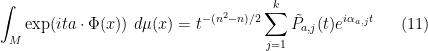
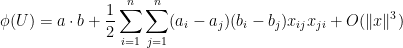
We now apply the Duistermaat-Heckman theorem to the task of proving the Harish-Chandra-Itzykson-Zuber integral formula. We first observe that it will suffice to establish the weaker formula


for any Hermitian , all complex , and some  depending only on
  . For, if this identity held, then by sending
  we see that the
  coefficient of the Taylor series of
  would equal
  . But we may expand this determinant as

so by Taylor expansion the coefficient is

where the outer summation is over all natural numbers  that sum to
  .
.
Consider a summand in which  for some
  . Then we see that this summand changes sign if we swap
  and
and  . For this reason we see that we may restrict attention to the case when the
  are all distinct; as the sum to
  , we conclude that is a permutation of
  . We can then rearrange the above sum as

which factorises as  , yielding the Harish-Chandra-Itzykson-Zuber integral formula.
It remains to prove (12). By unitary invariance we may take to be diagonal; by perturbation we may take the eigenvalues of to be generic (in, say, the Zariski sense), thus

and

for some  and
and  generic. By analytic continuation we may take to be imaginary. It will then suffice to show that

where  and
and  with distinct entries and all non-zero real , where
  depends only on
  . By subtracting a constant from we may take to be trace zero, and similarly for (and then generic relative to this constraint). The right-hand side can be expanded as

As for the left side, we introduce the coadjoint orbit

which, as the eigenvalues of are generic, is a smooth manifold of dimension  , which has a transitive action of on it. (Strictly speaking, is actually the rotation of a coadjoint orbit by , because the Lie algebra of is given by skew-Hermitian matrices rather than Hermitian matrices, but we will abuse notation by ignoring this distinction in the arguments that follow.) If we let
  be the diagonal map

then it thus suffices to show that

for all generic vectors  of trace zero, all non-zero , and some Haar measure
  on (i.e. a non-zero -invariant Radon measure), and some constant
  depending only on . Note that (7) is asserting an exact formula for the Fourier transform of the pushforward measure
  (or of its one-dimensional projection
  ).
).
Note that as is assumed to have trace zero, all elements of have trace zero as well, so actually takes values in the hyperplane  .
.
We now seek to interpret as a symplectic manifold and as a moment map for a torus action, in order to view as a Duistermmat-Heckman measure. We first need to construct a symplectic form on the coadjoint orbit , known as the Kirrilov-Kostant–Souriau form, as follows. Note that at any element of , the tangent vectors to at (which can be viewed as Hermitian matrices) take the form ![{[P,S]}](https://s0.wp.com/latex.php?latex=%7B%5BP%2CS%5D%7D&bg=ffffff&fg=000000&s=0&c=20201002) for some skew-Hermitian matrix
for some skew-Hermitian matrix  . The symplectic form
  at is then defined by the formula
![\displaystyle \omega(P)([P,S],[P,T]) := \hbox{tr}( i P [S,T] ). \ \ \ \ \ (8)](https://s0.wp.com/latex.php?latex=%5Cdisplaystyle+%5Comega%28P%29%28%5BP%2CS%5D%2C%5BP%2CT%5D%29+%3A%3D+%5Chbox%7Btr%7D%28+i+P+%5BS%2CT%5D+%29.+%5C+%5C+%5C+%5C+%5C+%288%29&bg=ffffff&fg=000000&s=0&c=20201002)
(The sign conventions are sometimes reversed in the literature; note that and ![{i[S,T]}](https://s0.wp.com/latex.php?latex=%7Bi%5BS%2CT%5D%7D&bg=ffffff&fg=000000&s=0&c=20201002) are Hermitian and so this expression is real-valued.) Using the cyclic properties of trace, we have the identity
are Hermitian and so this expression is real-valued.) Using the cyclic properties of trace, we have the identity
![\displaystyle \hbox{tr}(i P [S,T] ) = \hbox{tr}( i [P,S] T ) = - \hbox{tr}( i [P,T] S )](https://s0.wp.com/latex.php?latex=%5Cdisplaystyle+%5Chbox%7Btr%7D%28i+P+%5BS%2CT%5D+%29+%3D+%5Chbox%7Btr%7D%28+i+%5BP%2CS%5D+T+%29+%3D+-+%5Chbox%7Btr%7D%28+i+%5BP%2CT%5D+S+%29&bg=ffffff&fg=000000&s=0&c=20201002)
whence we see that the above form is well-defined (the dependence of ![{\hbox{tr}(iP[S,T])}](https://s0.wp.com/latex.php?latex=%7B%5Chbox%7Btr%7D%28iP%5BS%2CT%5D%29%7D&bg=ffffff&fg=000000&s=0&c=20201002) on factors through , and similarly for ). It is clearly a smooth anti-symmetric form, and is also invariant with respect to the conjugation action. By working with explicit matrix coefficients at
on factors through , and similarly for ). It is clearly a smooth anti-symmetric form, and is also invariant with respect to the conjugation action. By working with explicit matrix coefficients at  and using the hypotheses that the are distinct, one can soon verify that is non-degenerate at , and hence non-degenerate everywhere by the invariance. To verify that is a symplectic form, it remains to establish that is closed. This can be done by direct computation, but it turns out to be slicker to delay the verification of the symplectic nature of
  until some further facts about and have been established.
Now we express as a moment map (and, as a byproduct, conclude the closed nature of ). For any  , we consider the scalar map
  , which can be written as

Differentiating this along an arbitrary vector field ![{Y(P) = [P,S]}](https://s0.wp.com/latex.php?latex=%7BY%28P%29+%3D+%5BP%2CS%5D%7D&bg=ffffff&fg=000000&s=0&c=20201002) we see that
we see that
![\displaystyle d(a \cdot \Phi)(P)(Y) = \hbox{tr}( \hbox{diag}(a) [P,S] )](https://s0.wp.com/latex.php?latex=%5Cdisplaystyle+d%28a+%5Ccdot+%5CPhi%29%28P%29%28Y%29+%3D+%5Chbox%7Btr%7D%28+%5Chbox%7Bdiag%7D%28a%29+%5BP%2CS%5D+%29&bg=ffffff&fg=000000&s=0&c=20201002)

where  is the vector field
 ![{X_a(P) := [P, i \hbox{diag}(a)]}](https://s0.wp.com/latex.php?latex=%7BX_a%28P%29+%3A%3D+%5BP%2C+i+%5Chbox%7Bdiag%7D%28a%29%5D%7D&bg=ffffff&fg=000000&s=0&c=20201002) . As was arbitrary, we conclude that
. As was arbitrary, we conclude that

In particular,  is closed:

On the other hand, as is preserved by the action, and  is the vector field for the infinitesimal generator conjugation with respect to the unitary diagonal matrix
  for infinitesimal , we see that preserves :

Applying Cartan’s formula (5) we conclude that

for all . By unitary invariance again we conclude that  for any skew-Hermitian , where
 ![{X_A(P) := [P,A]}](https://s0.wp.com/latex.php?latex=%7BX_A%28P%29+%3A%3D+%5BP%2CA%5D%7D&bg=ffffff&fg=000000&s=0&c=20201002) . As the
. As the  span the tangent space, we obtain , and so is closed and thus symplectic as required.
Now that is known to be a symplectic manifold, we may form the Liouville measure  ; as is invariant under the conjugation action, is also, so this is a Haar measure. From (9) we From this we see that is the moment map for the conjugation action of the -dimensional torus of unitary diagonal matrices of determinant , after identifying with
  by taking the diagonal matrix entries and dividing by . This makes a Duistermaat-Heckman measure, and thus a multiple of Lebesgue measure on by polynomial of degree at most
  at every regular value of .
Now we work out what the regular values of are. If is a critical point of , then by the above calculations we must have ![{[P, i\hbox{diag}(a)] = 0}](https://s0.wp.com/latex.php?latex=%7B%5BP%2C+i%5Chbox%7Bdiag%7D%28a%29%5D+%3D+0%7D&bg=ffffff&fg=000000&s=0&c=20201002) for some non-trivial . The centraliser of a non-constant diagonal matrix consists of block diagonal matrices, so this only occurs when is block-diagonal. As has the same eigenvalues as , each block of then has eigenvalues that are a subset of
for some non-trivial . The centraliser of a non-constant diagonal matrix consists of block diagonal matrices, so this only occurs when is block-diagonal. As has the same eigenvalues as , each block of then has eigenvalues that are a subset of  . Taking partial traces, we then conclude that
  lies on a hyperplane of the form

for some  and some
  and
and  . Outside of these hyperplanes, we have regular points. The set of block diagonal matrices in can easily be verified to have zero measure (it has strictly lower dimension than ), so the Duistermaat-Heckman measure
  is thus a piecewise polynomial multiple of Lebesgue measure on which is smooth everywhere except at the hyperplanes (10). Note that these hyperplanes (10) partition into a finite number of polytopes. After performing a sequence of
  projections to spaces of one lower dimension, we conclude that (for generic ) the one-dimensional measure
  is also piecewise polynomial, with a finite number of pieces (supported on intervals) and the polynomial being of degree at most
  on each piece. (This fact can also be established directly from Proposition 1 in the case when is commensurate as well as generic.) In particular, if one differentiates (in the distributional sense) this one-dimensional measure
  times, one obtains a distribution that is supported on a finite number of points
  (depending on ), and so its Fourier transform takes the form
  for some polynomials
  . Undoing the differentiation, we thus conclude that
for some polynomials  and some distinct reals
  . This is already some way towards what our goal (7), but we still need to sort out exactly what the
  and
and  are. There are a number of ways to do this (e.g. one can use the Atiyah-Bott–Berline-Vergne localization theorem, or the machinery of symplectic cobordism), but we will use the method of stationary phase instead. The idea is to obtain an asympotic of the form

when  (keeping
  fixed); this asymptotic with the correct main term, combined with the expression (11) with a general main term but no error term, gives the formula (7) with the correct main term and no error term (the point being that it is not possible for an expression of the form
  to decay to zero at infinity without actually vanishing identically, as can be seen for instance by using frequency localisation operators to separate the contribution of each of the frequencies ).
It remains to establish (12). Up to a scalar multiple depending on , the left-hand side of (12) is equal to
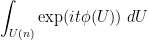
where  is the phase
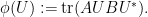
Following the method of statinonary phase, we now study how the stationary points of . Given a unitary matrix , an infinitesimal perturbation of it takes the form  for some skew-Hermitian matrix , and so the first variation of in this direction is
![\displaystyle \hbox{tr}( A U [X,B] U^* ) = \hbox{tr}( U^* A U [X,B] ).](https://s0.wp.com/latex.php?latex=%5Cdisplaystyle+%5Chbox%7Btr%7D%28+A+U+%5BX%2CB%5D+U%5E%2A+%29+%3D+%5Chbox%7Btr%7D%28+U%5E%2A+A+U+%5BX%2CB%5D+%29.&bg=ffffff&fg=000000&s=0&c=20201002)
As is diagonal with generic entries, ![{[X,B]}](https://s0.wp.com/latex.php?latex=%7B%5BX%2CB%5D%7D&bg=ffffff&fg=000000&s=0&c=20201002) ranges over the Hermitian matrices with zero diagonal, or equivalently the orthogonal complement of the diagonal Hermitian matrices with respect to the Hilbert-Schmidt inner product
ranges over the Hermitian matrices with zero diagonal, or equivalently the orthogonal complement of the diagonal Hermitian matrices with respect to the Hilbert-Schmidt inner product  . In order for to be stationary at , it is thus necessary and sufficient for
  to be diagonal, which (as is a generic diagonal matrix) only occurs when is a diagonal matrix. Thus we see that is only stationary at the permutation matrices
  , at which point it takes the value of
  .
.
Next, we expand to second order at each of its stationary points. We begin with an expansion near the identity matrix  . We use exponential coordinates
  , where is a small skew-Hermitian matrix, so that

Taylor expanding the exponential, we obtain

Writing 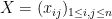 , this becomes
and hence by the skew-Hermitian nature of

We thus see that the Hessian of at in exponential coordinates has a determinant square root (using the branch in the upper half-plane, which is what is needed for the  asymptotics) which is
  for some absolute constant
  . Similarly, the determinant square root of the Hessian of at any other permutation matrix
  can be computed to be
  . Using stationary phase expansions (see e.g. Chapter IX of Stein’s “Harmonic analysis“) we obtain the desired expansion (12).


15 comments
Comments feed for this article
10 February, 2013 at 5:49 am
very small typo
I don’t understand this post at all,maybe I will never understand it .But I find a typo.In the first paragraph,
Let {A, B} be {n \times n} Hermitian matrices, with eigenvalues {\lambda_1(A) \leq \ldots \leq \lambda_n(A)} and {\lambda_1(B) \leq \ldots\leq \lambda_n(B)}.
“}” should be deleted……
[Corrected, thanks – T.]
10 February, 2013 at 8:53 pm
John
Dear terry,
It’s really nice to see duistermaat Heckman formula explained in such simple terms and with great elementary examples, and even a remarkable application. My only technical question concerns the formula partial_t[omega_p] – partial_t[omega_(p-t)] =0. How does that follow from the previous equation that the formula without square bracket is closed? Also want to mention that I learned the proof of HCIZ formula first from johansson’s paper on Gaussian divisible matrices.
John
[Oops, “closed” should be “exact” in that sentence; I’ve edited accordingly. -T.]
12 February, 2013 at 4:31 am
John
Thanks! I was worried that the exactness does not hold after quotient. But that seems to be the point of showing theta difference quantity is a pullback under the inclusion map.
13 February, 2013 at 7:44 am
Jean-Bernard Zuber
The presentation of Duistermaat-Heckman formula and its application to
HCIZ is very nice.
But I’m slightly puzzled by the other derivation, “Dyson Brownian
motion”. It seems to rely on Brezin-Hikami-Johansson formula,
which is itself using … HCIZ formula! Is the argument not circular ?
There is a slight variant, also starting from the group average of the
heat kernel on V_n, for which one derives after multiplication by
the Vandermonde determinant a heat equation in flat coordinates.
This is the method originally used by C. Itzykson and myself,
in J. Math. Phys. 21 (1980) 411-421. In that paper yet another
method, based on a character expansion and the Binet-Cauchy formula,
is given. And of course, there is a fourth derivation,
which is Harish-Chandra’s ! (a simple presentation of which I would
love to see …)
For the anecdote, we had already observed in 1979 that an
a priori totally unjustified
stationary phase approximation of the integral over the unitary
group was giving the right answer for small values of n ! This is what
prompted us to look for more robust derivations of that formula.
And the exactness of our stationary phase approximation was justified a
few years later, thanks to the D-H formula.
The Harish-Chandra formula is mentioned in DH’s paper. The application of
DH’s formula to HCIZ was later discussed in detail by Szabo,
arXiv:hep-th/9608068, and by many others.
Jean-Bernard Zuber
13 February, 2013 at 8:04 am
Terence Tao
Thanks for the references and early history of this result! I have adjusted the text accordingly.
Regarding the Brezin-Hikami-Johansson formula, in Johansson’s paper, two proofs of this formula are given. The first, as you say, uses the HCIZ formula and would thus of course be unusable for the purposes of this blog post. But the second proof (given in page 689 of that paper) proceeds by an analysis of Dyson Brownian Motion instead of HCIZ, and Johansson comments in that paper that one can use that proof to give a non-circular proof of HCIZ, basically along the lines given in this post. Of course, this is more or less what you do in your paper with Itzykson (the heat equation weighted by the Vandermonde determinant being essentially the Fokker-Planck equation for the Dyson Brownian motion), and is also the approach I took in this previous blog post about three years ago. So I guess the summary of the situation is that the HCIZ and Brezis-Hikami-Johansson formulae are logically equivalent to each other, and either formula can be proven by solving the relevant heat equation or Brownian motion.
13 February, 2013 at 1:23 pm
Jean-Bernard Zuber
Thanks a lot for this clarification. Incidentally, do not confuse Brezis, the
mathematician, and Brezin, the physicist. Here we are talking about
Edouard Brezin…
[Corrected, thanks – T.]
15 February, 2013 at 2:15 am
Paul Bubenzer
A more conceptual proof that is closed can be found in the proof of Lemma 7.22 of Berline/Getzler/Vergne’s “Heat Kernels and Dirac Operators”:
 is
is  -invariant.

 . Here,
  is the fundamental vector field associated to
  .
.
First, you need to establish that
Second, observe that the fundamental vector fields (i.e. the vector fields that arise from the infinitesimal action of an element of the lie algebra) span the tangent space of the coadjoint orbit at each point.
Third, you need to prove the defining equation of the momentum map, i.e. show that
holds for
Then we have
 .
. (by
(by  -invariance) and E. Cartan’s homotopy formula.
 , as desired.
The last equal sign follows from
As the fundamental vector fields span the tangent space, we have
16 February, 2013 at 11:39 am
Terence Tao
That’s a nice argument! I hadn’t realised that the moment map equation can be used even before one has fully verified that one has a symplectic structure. I’ve updated the text accordingly in order to incorporate this argument.
23 June, 2013 at 9:12 pm
jefferson alexander vitola
Hi Tao wrote you an email and never answered was more than 3 months ago
I asked you solve the definite integral of methods oscillatory
Integrate [(-8796541 * Pi ^ 12) / 322 * Sin [x ^ 4], {x, 74.37, 97.28}] or Integrate [(-8,796,541 * Pi ^ 12) / 322 * Sin [x * x * x * x], {x, 74.37, 97.28}]
and that your making the approximate with just pencil and paper and a pocket calculator,,,,, I hope do your answer,,,,clarified that the exercise proposed by my above,,, I do not need approximation of the number,,, I need are the procedures and series that you use to solve it, and that these series can be replaced in a pocket calculator,,,thanks
att
jefferson alexander vitola
att
jefferson alexander vitola
17 August, 2017 at 10:10 pm
On the sign patterns of entrywise positivity preservers in fixed dimension | What's new
[…] with a geometric miracle, namely the Harish-Chandra-Itzykson-Zuber identity, which I discussed in this previous blog post. This factors the above generalised Vandermonde determinant as the product of the ordinary […]
14 December, 2017 at 6:44 am
pietro rotondo
Dear Terence,
we noticed that the HCIZ formula holds also for degenerate eigenvalues of either matrices A and B. However in this case, both the numerator and the denominator are zero and an implicit cancellation occurs. Do you know whether a close formula exists once the cancellation has been explicitly performed?
Best Regards
Pietro Rotondo
14 December, 2017 at 9:55 am
Jean-Bernard Zuber
Well, you may Taylor expand the rows of the determinant that have coalescing arguments. Suppose that tend to
  , while
 ‘s are fixed.
 reading
  , the other rows as usual,
 ‘s times the Vandermonde of the non coalescing
  ‘s.
‘s.
the others and the
You’ll get a determinant with rows 1 to
divided by the Vandermonde of the
1 January, 2018 at 5:07 pm
lizhongyangmath
Should there be a factor on the right hand side of on the right hand side of the equation below “Comparing this against (3)”?
[Corrected, thanks – T.]
21 February, 2018 at 5:49 am
Anonymous
It’s a minor thing, but isn’t there a problem with signs in examples 1 and 2? The flow of the hamiltonian vector field is clockwise, while a complex number will rotate anticlockwise when multiplied by a number like exp(it).
[Corrected, thanks – T.]
7 April, 2022 at 2:10 am
inequalities - Nonnegativity locus of Schur polynomials Answer - Lord Web
[…] means that some Fourier evaluation could breathe helpful for the common illustration, or maybe the Harish-Chandra-Itzykson-Zuber methodhowever I do not know how you can refer about […]