[These are notes intended mostly for myself, as these topics are useful in random matrix theory, but may be of interest to some readers also. -T.]
One of the most fundamental partial differential equations in mathematics is the heat equation
where  is a scalar function
  of both time and space, and
  is the Laplacian
  . For the purposes of this post, we will ignore all technical issues of regularity and decay, and always assume that the solutions to equations such as (1) have all the regularity and decay in order to justify all formal operations such as the chain rule, integration by parts, or differentiation under the integral sign. The factor of
  in the definition of the heat propagator is of course an arbitrary normalisation, chosen for some minor technical reasons; one can certainly continue the discussion below with other choices of normalisations if desired.
In probability theory, this equation takes on particular significance when  is restricted to be non-negative, and furthermore to be a probability measure at each time, in the sense that
for all  . (Actually, it suffices to verify this constraint at time
  , as the heat equation (1) will then preserve this constraint.) Indeed, in this case, one can interpret
  as the probability distribution of a Brownian motion
where  is a stochastic process with initial probability distribution
  ; see for instance this previous blog post for more discussion.
A model example of a solution to the heat equation to keep in mind is that of the fundamental solution

defined for any  , which represents the distribution of Brownian motion of a particle starting at the origin
  at time . At time ,
  represents an
  -valued random variable, each coefficient of which is an independent random variable of mean zero and variance . (As
  ,
,  converges in the sense of distributions to a Dirac mass at the origin.)
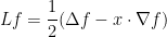
The heat equation can also be viewed as the gradient flow for the Dirichlet form
since one has the integration by parts identity

for all smooth, rapidly decreasing  , which formally implies that
  is (half of) the negative gradient of the Dirichlet energy
  with respect to the
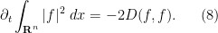
  inner product. Among other things, this implies that the Dirichlet energy decreases in time:
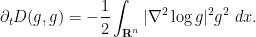
For instance, for the fundamental solution (3), one can verify for any time that
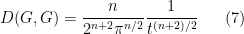
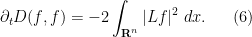
(assuming I have not made a mistake in the calculation). In a similar spirit we have
Since  is non-negative, the formula (6) implies that
  is integrable in time, and in particular we see that
  converges to zero as
  , in some averaged
  sense at least; similarly, (8) suggests that also converges to zero. This suggests that converges to a constant function; but as is also supposed to decay to zero at spatial infinity, we thus expect solutions to the heat equation in to decay to zero in some sense as . However, the decay is only expected to be polynomial in nature rather than exponential; for instance, the solution (3) decays in the
  norm like
  .
.
Since  , we also observe the basic cancellation property

for any function .
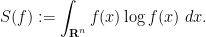
There are other quantities relating to that also decrease in time under heat flow, particularly in the important case when is a probability measure. In this case, it is natural to introduce the entropy
Thus, for instance, if  is the uniform distribution on some measurable subset
  of of finite measure
  , the entropy would be
  . Intuitively, as the entropy decreases, the probability distribution gets wider and flatter. For instance, in the case of the fundamental solution (3), one has
 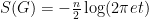 for any , reflecting the fact that is approximately uniformly distributed on a ball of radius
  (and thus of measure
  ).
).
A short formal computation shows (if one assumes for simplicity that is strictly positive, which is not an unreasonable hypothesis, particularly in view of the strong maximum principle) using (9), (5) that
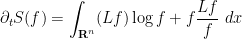


where  is the square root of . For instance, if is the fundamental solution (3), one can check that
  (note that this is a significantly cleaner formula than (7)!).
In particular, the entropy is decreasing, which corresponds well to one’s intuition that the heat equation (or Brownian motion) should serve to spread out a probability distribution over time.
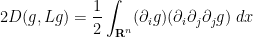
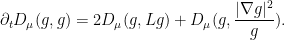
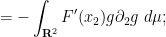
Actually, one can say more: the rate of decrease  of the entropy is itself decreasing, or in other words the entropy is convex. I do not have a satisfactorily intuitive reason for this phenomenon, but it can be proved by straightforward application of basic several variable calculus tools (such as the chain rule, product rule, quotient rule, and integration by parts), and completing the square. Namely, by using the chain rule we have

valid for for any smooth function  , we see from (1) that
and thus (again assuming that , and hence  , is strictly positive to avoid technicalities)

We thus have
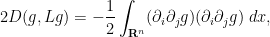
It is now convenient to compute using the Einstein summation convention to hide the summation over indices  . We have
and
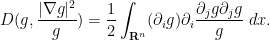
By integration by parts and interchanging partial derivatives, we may write the first integral as
and from the quotient and product rules, we may write the second integral as

Gathering terms, completing the square, and making the summations explicit again, we see that

and so in particular  is always decreasing.
The above identity can also be written as
Exercise 1 Give an alternate proof of the above identity by writing  ,
,  and deriving the equation
 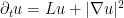 for
for  .
.
It was observed in a well known paper of Bakry and Emery that the above monotonicity properties hold for a much larger class of heat flow-type equations, and lead to a number of important relations between energy and entropy, such as the log-Sobolev inequality of Gross and of Federbush, and the hypercontractivity inequality of Nelson; we will discuss one such family of generalisations (or more precisely, variants) below the fold.
We modify the above examples by replacing the Lebesgue measure  on by a probability measure
  , which (inspired by the formalism of statistical mechanics) is customarily written in the form
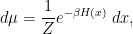
where the Hamiltonian  is some (smooth) function that grows at a suitable rate at infinity (to make
  have finite mass),
  is a scaling parameter (sometimes referred to as the inverse temperature), and
  is a normalisation constant (known as the partition function). A model example here is that of the Gaussian distribution

which would correspond to the harmonic oscillator Hamiltonian 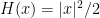 with
with  , or of a random Gaussian vector in which each coefficient independently has a normal distribution of mean zero and variance one. (For the purposes of this blog post, one could combine the
  and
and  quantities into a single object if one wished, effectively normalising to equal
  , but there can be some minor advantages to using a different normalisation to for some applications, for instance if one is interested in large dimensional limits
  .)
.)
While we are altering the base measure here, we will retain the Euclidean gradient structure; one can of course consider even more general variants of heat flow (such as heat flow on Riemannian manifolds) in which we also change the gradient structure; these are also of interest for many applications, but we will not consider them here.
We can form the Dirichlet form  relative to (but retaining the Euclidean gradient structure, as mentioned above) by the formula

in analogy with (4). In analogy with (5), we then have

where is the differential operator
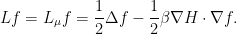
For instance, in the Gaussian case (11), becomes the Ornstein-Uhlenbeck operator
(note that the normalisation factor of is not always present in the literature concerning this operator). Observe that (or equivalently, that  for all reasonable ) and so from (12) we have the analogue of (9), namely that

for all (smooth, not too rapidly increasing) .
The corresponding gradient flow (now using the inner product structure of  , rather than
  ) is then
This equation becomes probabilistically meaningful if  is a probability measure, thus is non-negative and

for all times (but again, it is easy to see using (13) that if this constraint holds for one time, it holds for all subsequent times also). In probabilistic terms, the probability measure  then represents the probability distribution at time of a particle
  with initial distribution
  at time zero, and obeying the stochastic differential equation
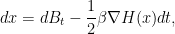
which can be viewed as a combination of Brownian motion  and gradient flow
  . For instance, in the Gaussian case (11), this equation becomes the Ornstein-Uhlenbeck process
with the relative density then obeying the Ornstein-Uhlenbeck equation
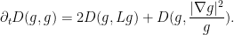
As before, we have a number of monotonicity formulae for the heat flow (14), such as

and
which strongly suggests (as before) that should be converging as to a function with  , i.e. to a constant function. In particular, as is normalised to be a probability measure, and is also a probability measure, then we expect to converge to .
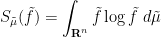
One way to quantify this convergence is to introduce the entropy

If and are both probability measures, then a simple application of Jensen’s inequality gives us that  is non-negative. Indeed, we can say more:
Lemma 1 (Entropy controls total variation) We have  .
.
This inequality is also known as Pinsker’s inequality.
Proof: We first give a crude argument that loses a factor of  . As
. As  has a second derivative of
  , we see from Taylor expansion at that
for any  , and hence on replacing
  by
by  and integrating against , we see that

and hence by Cauchy-Schwarz

and hence since has mean with respect to

which on squaring gives the bound with a loss of . To eliminate the loss, we use an argument of Kemperman (which also appears in a subsequent paper of Diaconis and Saloff-Coste), and use the more precise inequality

which can be verified by elementary calculus (indeed, this function vanishes to fourth order at  and has the non-negative second derivative of
  ). We then conclude that

since  , the claim then follows from the Cauchy-Schwarz inequality.
The computations used to compute the time derivative of  also work for , leading to the identity

where  . The formula for the time derivative for
  is a bit more interesting. The chain rule (10) still holds for (why?), and so we still have
and thus
As in the Euclidean case, we have

The situation with  is however a bit more complicated:

If we perform integration by parts on the first integral, it becomes

this partially cancels the second integral, leading to the formula

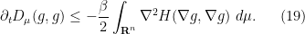
Combining this with (18) and completing the square as in the Euclidean case, we conclude that

where  is the Hessian of :

In particular, we have the Bakry-Emery inequality
If is convex, then this implies that is non-increasing, much as in the Euclidean case. However, the situation improves significantly if is (uniformly) strictly convex in the sense that
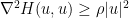
for some fixed  . In this case, we have

and thus by Gronwall’s inequality we have the exponential decay

for all  . This suggests that (and hence ) relaxes exponentially fast to the equilibrium state , with the time of relaxation being of the order of
  . In particular, we expect to converge to
  as . From (17) and the fundamental theorem of calculus we therefore have (formally at least) that

and hence from (20) we have the log-Sobolev inequality

or to put in a more familiar way, we have

whenever  .
.
Exercise 2 Formally establish the exponential decay of entropy

whenever is a probability measure obeying the heat equation (14).
In the gaussian case (11), we have  , and (21) is the classical log-Sobolev inequality of Gross and of Federbush. But we see from the above argument that log-Sobolev inequalities in fact hold for all convex Hamiltonians .
Exercise 3 Using (21), formally establish the hypercontractivity inequality

whenever is a non-negative solution to the heat flow (14). (Hint: compute the derivative of  at some time
  , after performing the normalisation
  .) Conversely, show that the hypercontractivity inequality (22) implies the log-Sobolev inequality (21). In the Gaussian case (11), the hypercontractivity inequality is due to Nelson; the equivalence between the two inequalities was first observed by Federbush.
Log-Sobolev inequalities can also be used to establish concentration of measure inequalities; see for instance this previous blog post for an instance of this.
The exponential convergence to equilibrium in the convex case should be contrasted with the polynomial convergence to zero in the Euclidean case. As always, the model gaussian case (11) is instructive. Let us use the Brownian motion formalism. In the Euclidean case, using the Brownian motion (2), and assuming mean zero  for simplicity, we have constant variance production thanks to Ito’s formula
  :
:
On the other hand, with the Ornstein-Uhlenbeck process (15) with mean zero, a short computation shows that the variance instead obeys the formula

and thus  relaxes exponentially fast to the identity. One can also see this from the explicit solution

to the Ornstein-Uhlenbeck equation (16).
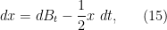
The exponential convergence to equilibrium can also be understood as a probabilistic mixing inequality. Let us take the model case of a quadratic Hamiltonian attaining a minimum at  :
:
In this case, the stochastic equation is a more general Ornstein-Uhlenbeck process

The natural length scale for the measure is  , since the weight starts decreasing faster than exponentially once one wanders more than this length scale away from the Hamiltonian minimiser . The natural scale for the drift velocity
  is thus
  . Over a time scale
  , the net drift should then be
  , while the net diffusion from the Brownian motion component
  of the process should be
  . The two contributions meet at
  , which helps explain why this is the mixing time for relaxation to equilibrium; it is basically the time needed for the random portion of the dynamics to fill out the space drawn by the equilibrium.
The above Bakry-Emery theory works well when the Hamiltonian is “isotropic” in the sense that it has about the same amount of convexity in any direction (or to put it another way, the Hessian is well-conditioned), as was the case in the quadratic examples (23). But it does not give completely satisfactory results for “non-isotropic” choices of Hamiltonian. A simple example is provided by the two-dimensional anisotropic quadratic Hamiltonian

for some  with ; this corresponds to two decoupled Ornstein-Uhlenbeck process, a “slow” process

which takes time  to converge to equilibrium, and an independent “fast” process

which takes the shorter time of  to converge to equilibrium. One should view
  as a “macroscopic” or “global” coordinate of a system, while
  is a “microscopic” or “local” coordinate. We have the strict convexity bound

which by the above theory gives convergence to equilibrium of the combined process  in time . This is the right order of magnitude if one is interested in convergence to global equilibrium, but it does not capture the fact that convergence to local equilibrium (as measured by convergence of the component) can occur at times much sooner than . However, in a series of papers by Erdos, Schlein, Yau, and Yin (see also these later surveys), the local relaxation flow method were developed to improve upon the basic Bakry-Emery theory, with applications to the universality theory of random matrices. We can illustrate some of the basic ideas of this method with the simple example of the decoupled Hamiltonian (24) (though the whole point of the method, for the purpose of applications, is that it can also be applied to more complicated Hamiltonians in which the slow and fast modes are coupled together).
The first trick is to refrain from applying the inequality (25) to the Bakry-Emery inequality (19) as it is too lossy in the fast variables. Instead, since
we see that (19) implies that

Integrating this, we obtain an additional bound on  which becomes useful in the regime when
  is much larger than
  :
:

This gives some additional smoothing in the direction. For instance, given a test function  of the variable only, we have


since  , we thus have from Cauchy-Schwarz that

integrating this from to some time  and using Cauchy-Schwarz again followed by, we see that

Given that the time to relaxation to equilibrium is , we morally have  for
for  , so heuristically at least we have the bound

For sake of comparison, the log-Sobolev inequality (21) followed by Lemma 1 gives a bound of the shape

for all  (which can now depend on as well as ). The bound (27) is better than the log-Sobolev bound when the test function is spread out over scales larger than the natural length scale
  of the fast variable. This suggests that such statistics are universal among all distributions for which one can control the Dirichlet functional
  . (In the context of the theory of universality theory for Wigner random matrices, this corresponds to local spectral statistics that have been averaged in the energy parameter in order to reduce the dependence of these statistics on fast variables.)
The above trick improves the estimates somewhat, but it still involves the slow relaxation time  , which is undesirable for some applications. The second trick in the method of local relaxation flow is to modify the Hamiltonian, working with a more convexified (but slightly artificial) Hamiltonian
  , such as

for some parameter  , which one can think of as being intermediate between and for our toy example. Since
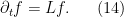
 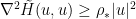 , Bakry-Emery theory tells us that the associated heat equation
  associated to this modified Hamiltonian (which Erdos, Schlein, Yau, and Yin refer to as the local relaxation flow) will relax to a local equilibrium measure
  in time
  , which can be considerably faster than the relaxation time to global equilibrium if the parameter is chosen appropriately. In particular, this can lead to improvements in the constants for bounds such as (27) (namely, by replacing there with ), at the cost of replacing the original Dirichlet energy
  with a modified Dirichlet energy
  .
.
Of course, in practice one is not directly interested in the local relaxation flow, but in solutions to the original heat equation  . As such, the Bakry-Emery inequality (19) for such flows does not directly say much about the modified Dirichlet energy
  , as it only directly controls the original Dirichlet energy (and in practice, the ratio between and will be quite large). Nevertheless, one can adapt the Bakry-Emery methods to say something useful in this setting. Starting with a solution to the original heat equation
  , we define a modified function
  by the formula

In other words, we have  , where
  is the weight
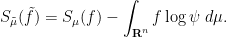
  . Instead of working with the entropy
  of relative to , we instead work with the entropy
of with respect to ; we may write this as
Differentiating this using (17), one has
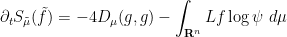
where  . We easily verify using (12), (10) that


Meanwhile,  , we have
  , and so


and thus on combining these identities and simplifying, we see that
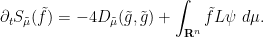
We can write the second term as

but from (13) one has

and thus

If is related to by (28) with , then

and so

To remove the derivative here, we can apply the arithmetic mean-geometric mean inequality to obtain

and so

In many applications, one can get good control on the variance  ; in the context of universality for Wigner matrices, such bounds can be obtained from local semi-circular laws, and particularly from a strong version of such a law, known as eigenvalue rigidity. Because of this, one can get good bounds on the entropy
  and Dirichlet form
  with respect to the local equilibrium measure in these cases in timescales as short as ; see for instance this survey of Erdos and Yau for details.
One of the main applications of the local relaxation flow method is to obtain universality for various local statistics of random matrices after averaging in the energy parameter. In some cases (notably in that of complex Wigner matrices that match the GUE ensemble to second order) it is possible to remove the energy averaging by using methods based on explicit formulae for the correlation functions, rather than by the local relaxation flow method; this was first achieved for certain classes of ensembles by Johansson, and later extended to increasingly wider sets of ensembles by many authors. However, it appears difficult to obtain such fixed-energy results from heat flow methods alone, as there is an insufficient amount of concentration of measure for the fixed-energy measurements. However, by combining these methods with (a variant of) the Holder continuity theory of parabolic equations of Caffarelli, Chan, and Vasseur, Erdos and Yau were recently able to obtain universality for a slightly different statistic, namely a fixed gap  between eigenvalues, without any averaging in the
  parameter. This avoids the need for energy averaging, but on the other hand the statistic studied is invariant with respect to the slow mode in which all the eigenvalues are translated by the same amount. It remains a technical challenge to discover a technique for understanding statistics that are not invariant (or nearly invariant) with respect to the slow mode, which does not invoke either explicit formulae or energy averaging.


11 comments
Comments feed for this article
6 February, 2013 at 8:46 am
hanbangxian
I am not sure if the problem you mentioned for random graph has relationship with the Ricci curvature of a graph.
7 February, 2013 at 8:00 am
d
I think your definition of entropy has the opposite sign to the standard one.
7 February, 2013 at 8:16 am
Terence Tao
Actually, relative entropy is usually defined using the positive sign (which, among other things, makes this quantity non-negative), in contrast to Shannon entropy or thermodynamic entropy which usually has the negative sign.
11 February, 2013 at 10:28 am
Djalil
Dear Terry,
regarding the sharp inequality for the proof of the optimal entropy-total-variation comparison, I though that it goes back at least to Kemperman (1969) http://www.ams.org/mathscinet-getitem?mr=252112 pages 2174-2175. It seems to me also that the inequality is often referred to as the Pinsker or Csiszár-Kullback inequality.
Best.
[Reference added, thanks – T.]
11 February, 2013 at 2:38 pm
Djalil
Precision: the first know proof is due to Pinsker (1963 or 64). However, the argument using the lower bound with a rational fraction is due to Kemperman (1969)… Best.
[Corrected, thanks – T.]
24 July, 2013 at 10:58 am
salazar
In the display above (19), the quadratic form should be defined by in Einstein convention, where
  and
and  are vectors?
[Corrected, thanks – T.]
28 September, 2014 at 7:49 pm
FC7
For your question “I do not have a satisfactorily intuitive reason for this phenomenon, but it can be proved by”. I think we have a partial answer for it. In a paper, we prove that the the third order derivative of S(f) is >=0 and the fourth order <=0. The paper can be found in arXiv: http://arxiv.org/abs/1409.5543
I have also sent an email to you.
20 September, 2015 at 11:30 am
Entropy and rare events | What's new
[…] this previous blog post for a proof of this inequality.) A standard application of Jensen’s inequality reveals that […]
30 December, 2020 at 5:13 pm
Anonymous
I check the result of equation (7),I think it should be 2^( n/2) in the denominator
[I believe the exponent is correct as stated – T.]
13 March, 2022 at 2:32 pm
TK
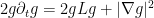
After eqn 10, you consider 2g d_t g for which one expression is 2g Lg by eqn 1. But another expression that you use is d_t g^2 = L g^2 and then appeal to eqn 10 to get 2gLg + |\nabla g|^2. But this would imply |\nabla g|^2 = 0 which seems wrong. Not sure what mistake I made….
13 March, 2022 at 9:31 pm
TK
Oh I got the issue. Nevermind.