Consider the free Schrödinger equation in  spatial dimensions, which I will normalise as
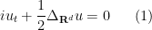
where  is the unknown field and
  is the spatial Laplacian. To avoid irrelevant technical issues I will restrict attention to smooth (classical) solutions to this equation, and will work locally in spacetime avoiding issues of decay at infinity (or at other singularities); I will also avoid issues involving branch cuts of functions such as
  (if one wishes, one can restrict to be even in order to safely ignore all branch cut issues). The space of solutions to (1) enjoys a number of symmetries. A particularly non-obvious symmetry is the pseudoconformal symmetry: if
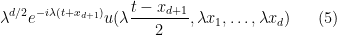
  solves (1), then the pseudoconformal solution
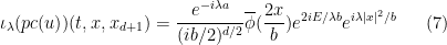
  defined by

for  can be seen after some computation to also solve (1). (If has suitable decay at spatial infinity and one chooses a suitable branch cut for
  , one can extend
  continuously to the
  spatial slice, whereupon it becomes essentially the spatial Fourier transform of
  , but we will not need this fact for the current discussion.)
An analogous symmetry exists for the free wave equation in  spatial dimensions, which I will write as
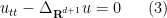
where  is the unknown field. In analogy to pseudoconformal symmetry, we have conformal symmetry: if solves (3), then the function
  , defined in the interior
  of the light cone by the formula

also solves (3).
There are also some direct links between the Schrödinger equation in dimensions and the wave equation in dimensions. This can be easily seen on the spacetime Fourier side: solutions to (1) have spacetime Fourier transform (formally) supported on a -dimensional hyperboloid, while solutions to (3) have spacetime Fourier transform formally supported on a -dimensional cone. To link the two, one then observes that the -dimensional hyperboloid can be viewed as a conic section (i.e. hyperplane slice) of the -dimensional cone. In physical space, this link is manifested as follows: if solves (1), then the function  defined by

solves (3). More generally, for any non-zero scaling parameter  , the function
  defined by

solves (3).
As an “extra challenge” posed in an exercise in one of my books (Exercise 2.28, to be precise), I asked the reader to use the embeddings  (or more generally
  ) to explicitly connect together the pseudoconformal transformation
  and the conformal transformation
  . It turns out that this connection is a little bit unusual, with the “obvious” guess (namely, that the embeddings intertwine and ) being incorrect, and as such this particular task was perhaps too difficult even for a challenge question. I’ve been asked a couple times to provide the connection more explicitly, so I will do so below the fold.
To state the connection, it turns out that one must first use separation of variables and restrict to a subclass of solutions to (1), namely those of the form

for some energy level  and some function
  . (The function
  then obeys the time-independent Schrödinger equation
 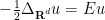 , although we will not use this equation here.) The connection between and is then as follows:
Proposition 1 Let be a solution to (1) of the form (6) for some energy  . Then we have

for any non-zero .
Thus, the conformal transformation is not intertwined with the pseudoconformal transformation via the embeddings  , but instead the conformal transformation relates different embeddings of the pseudoconformal transform of a solution to (1) to each other, where the precise embeddings involved depend on the energy level of the original solution .
We can verify this proposition by a straightforward calculation. From (6) and (2) we have

and thus by (5)
where we abbreviate 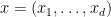 and also introduce the null coordinates
  ,
,  . Applying (4) and noting that
  , we conclude that

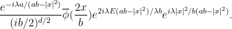
is equal to

We can cancel out the factors of  to get
Next, we can combine

to simplify the previous expression as
which we can rearrange a little as
Comparing this with (7), we see that this expression is equal to  as desired.


7 comments
Comments feed for this article
14 February, 2013 at 6:13 pm
samuelprime
The pseudoconformal transform has the look of the inversion formula for theta functions! Since the free Schrodinger equation is linear it’s enough to check that it can in fact hold for each exponential term involved in theta functions (with suitable choice of constants). So it is interesting that the inversion formula also holds for all solutions to the free Schrodinger equation. Very nice post.
14 February, 2013 at 10:49 pm
Mokhtar KIRANE
Please see
http://www3.imperial.ac.uk/newsandeventspggrp/imperialcollege/newssummary/news_17-6-2009-11-29-18?newsid=69042
15 February, 2013 at 8:44 pm
Marcelo de Almeida
Mokhtar KIRANE what is this?
22 February, 2013 at 8:51 am
Anonymous
I don’t know how my name came to this place
I have no interest in the subject
22 February, 2013 at 9:12 am
Marcelo de Almeida
ok
15 February, 2013 at 10:35 pm
samuelprime
Maybe worthwhile noting that both pc and conf are order 2 symmetries. So, pc(pc(u)) = u for any function u (even if it doesn’t satisfy the Schrodinger equation). (You may need to add a condition so the transform of u is again defined in the required domain R x R^d.) The same is the case for the conformal symmetry: conf(conf(u)) = u for each u. In view of what I said about theta functions (and which I didn’t state properly in my previous post) they are now invariant functions of pc — so are of pc-eigenvalue 1 (if you choose the parameter constants appropriately in the theta functions). Therefore functions can be decomposed into a sum of an invariant u and one of pc-eigenvalue -1. Proposition 1 (in Terry’s post) shows that these two order 2 symmetries interact in some subtle way. Do you know what pc(conf(u)) is? And how perhaps it could be related to conf(pc) given by Proposition 1? Might give an interesting commutation relation between the two symmetries of order 2.
4 April, 2013 at 7:04 pm
Sun's World
how to make a box around proposition 1?
[Custom CSS – see https://terrytao.wordpress.com/about/ -T. ]