This is the second thread for the Polymath8b project to obtain new bounds for the quantity
either for small values of  (in particular
  ) or asymptotically as
  . The previous thread may be found here. The currently best known bounds on
  are:
are:
- (Maynard)
 .
.
- (Polymath8b, tentative)
 .
.
- (Polymath8b, tentative)
 for sufficiently large .
- (Maynard) Assuming the Elliott-Halberstam conjecture,
 ,
,  , and
, and  .
.
Following the strategy of Maynard, the bounds on proceed by combining four ingredients:
- Distribution estimates
![{EH[\theta]}](https://s0.wp.com/latex.php?latex=%7BEH%5B%5Ctheta%5D%7D&bg=ffffff&fg=000000&s=0&c=20201002) or
or ![{MPZ[\varpi,\delta]}](https://s0.wp.com/latex.php?latex=%7BMPZ%5B%5Cvarpi%2C%5Cdelta%5D%7D&bg=ffffff&fg=000000&s=0&c=20201002) for the primes (or related objects);
for the primes (or related objects);
- Bounds for the minimal diameter
 of an admissible
  -tuple;
- Lower bounds for the optimal value
 to a certain variational problem;
- Sieve-theoretic arguments to convert the previous three ingredients into a bound on .
Accordingly, the most natural routes to improve the bounds on are to improve one or more of the above four ingredients.
Ingredient 1 was studied intensively in Polymath8a. The following results are known or conjectured (see the Polymath8a paper for notation and proofs):
- (Bombieri-Vinogradov) is true for all
 .
.
- (Polymath8a) is true for
 .
.
- (Polymath8a, tentative) is true for
 .
.
- (Elliott-Halberstam conjecture) is true for all
 .
.
Ingredient 2 was also studied intensively in Polymath8a, and is more or less a solved problem for the values of of interest (with exact values of for  , and quite good upper bounds for for
  , available at this page). So the main focus currently is on improving Ingredients 3 and 4.
For Ingredient 3, the basic variational problem is to understand the quantity

for  bounded measurable functions, not identically zero, on the simplex

with  being the quadratic forms

and

Equivalently, one has

where  is the positive semi-definite bounded self-adjoint operator

so is the operator norm of  . Another interpretation of
  is that the probability that a rook moving randomly in the unit cube
 ![{[0,1]^k}](https://s0.wp.com/latex.php?latex=%7B%5B0%2C1%5D%5Ek%7D&bg=ffffff&fg=000000&s=0&c=20201002) stays in simplex
stays in simplex  for
for  moves is asymptotically
  .
.
We now have a fairly good asymptotic understanding of , with the bounds

holding for sufficiently large . There is however still room to tighten the bounds on for small ; I’ll summarise some of the ideas discussed so far below the fold.
For Ingredient 4, the basic tool is this:
Theorem 1 (Maynard) If is true and  , then
  .
.
Thus, for instance, it is known that  and
and  , and this together with the Bombieri-Vinogradov inequality gives
  . This result is proven in Maynard’s paper and an alternate proof is also given in the previous blog post.
We have a number of ways to relax the hypotheses of this result, which we also summarise below the fold.
— 1. Improved sieving —
A direct modification of the proof of Theorem 1 also shows:
Theorem 2 If is true and ![{M_k({\cal R}_k \cap [0,\frac{\delta}{1/4+\varpi}]^k) > \frac{m}{1/4+\varpi}}](https://s0.wp.com/latex.php?latex=%7BM_k%28%7B%5Ccal+R%7D_k+%5Ccap+%5B0%2C%5Cfrac%7B%5Cdelta%7D%7B1%2F4%2B%5Cvarpi%7D%5D%5Ek%29+%3E+%5Cfrac%7Bm%7D%7B1%2F4%2B%5Cvarpi%7D%7D&bg=ffffff&fg=000000&s=0&c=20201002) , then .
, then .
Here is defined for the truncated simplex ![{{\cal R}_k \cap [0,\frac{\delta}{1/4+\varpi}]^k}](https://s0.wp.com/latex.php?latex=%7B%7B%5Ccal+R%7D_k+%5Ccap+%5B0%2C%5Cfrac%7B%5Cdelta%7D%7B1%2F4%2B%5Cvarpi%7D%5D%5Ek%7D&bg=ffffff&fg=000000&s=0&c=20201002) in the obvious fashion. This allows us to use the MPZ-type bounds obtained in Polymath8a, at the cost of requiring the test functions
in the obvious fashion. This allows us to use the MPZ-type bounds obtained in Polymath8a, at the cost of requiring the test functions  to have somewhat truncated support. Fortunately, in the large setting, the functions we were using had such a truncated support anyway. It looks likely that we can replace the cube
 ![{[0,\frac{\delta}{1/4+\varpi}]^k}](https://s0.wp.com/latex.php?latex=%7B%5B0%2C%5Cfrac%7B%5Cdelta%7D%7B1%2F4%2B%5Cvarpi%7D%5D%5Ek%7D&bg=ffffff&fg=000000&s=0&c=20201002) by significantly larger regions by using the (multiple) dense divisibility versions of
by significantly larger regions by using the (multiple) dense divisibility versions of  , but we have not yet looked into this.
It also appears that if one generalises the Elliott-Halberstam conjecture to also encompass more general Dirichlet convolutions  than the von Mangoldt function
  (see e.g. Conjecture 1 of Bombieri-Friedlander-Iwaniec), then one can enlarge the simplex in Theorem 1 (and probably for Theorem 2 also) to the slightly larger region

Basically, the reason for this is that the restriction to the simplex (as opposed to  ) is only needed to control the sum
  , but by splitting
  into products of simpler divisor sums, and using the Elliott-Halberstam hypothesis to control one of the factors, it looks like one can still control error terms in the larger region (but this will have to be checked at some point, if we end up using this refinement). This is only likely to give a slight improvement, except when is small; from the inclusions
and a scaling argument we see that
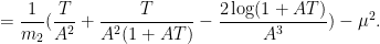
Assume EH. To improve the bound to  , it suffices to obtain a bound of the form

where
and
With given in terms of a cutoff function , the left-hand side  can be computed as usual as
while we have the upper bound


and other bounds may be possible. (This is discussed in this comment.)
For higher , it appears that similar maneuvers will have a relatively modest impact, perhaps shaving  or so off of the current values of .
— 2. Upper bound on —
We have the upper bound

for any  . To see this, observe from Cauchy-Schwarz that


The final factor is  , and so

Summing in and noting that  on the simplex we have

and the claim follows.
Setting  , we conclude that

for sufficiently large . There may be some room to improve these bounds a bit further.
— 3. Lower bounds on —
For small , one can optimise the quadratic form

by specialising to a finite-dimensional space and then performing the appropriate linear algebra. It is known that we may restrict without loss of generality to symmetric ; one could in principle also restrict to the functions of the form

for some symmetric function  (indeed, morally at least should be an eigenfunction of ), although we have not been able to take much advantage of this yet.
For large , we can use the bounds

for any  and any with
  ; we can also start with a given and improve it by replacing it with
  (normalising in
  if desired), and perhaps even iterating and accelerating this process.
The basic functions we have been using take the form

where
![\displaystyle g(t) := 1_{[0,T]} \frac{1}{1+AT}](https://s0.wp.com/latex.php?latex=%5Cdisplaystyle++g%28t%29+%3A%3D+1_%7B%5B0%2CT%5D%7D+%5Cfrac%7B1%7D%7B1%2BAT%7D&bg=ffffff&fg=000000&s=0&c=20201002)
and


Then , and

where  are iid random variables on
 ![{[0,T]}](https://s0.wp.com/latex.php?latex=%7B%5B0%2CT%5D%7D&bg=ffffff&fg=000000&s=0&c=20201002) with density
with density  . By Chebyshev’s inequality we then have

if  , where
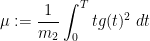

and
A lengthier computation for  gives
gives


assuming  .
.


129 comments
Comments feed for this article
22 November, 2013 at 7:51 pm
Terence Tao
It might be time to start collecting upper and lower bounds for for small k (say, up to k=105) to get a sense of how much room there is for improvement here, and what one can hope to achieve from the MPZ estimates (or from using fancier symmetric functions). The fact that
  is now known to not grow any faster than
  is a little disappointing for the large
  theory, but perhaps there is yet another way to modify the sieve to break this barrier (much as the GPY sieve, for which M_k never exceeded 4, was modified into the current sieve introduced by James). The only “hard” obstruction I know of is the parity obstruction, which basically stems from the belief that
  is negligible for just about any sieve under consideration, which means in probabilistic terms that
and in particular
This translates to the trivial bound in the current context, which is well short of the truth; it seems there is a substantial gap between “having an odd number of prime factors” and “is prime” when is working with k-tuple sieves.
22 November, 2013 at 9:24 pm
Pace Nielsen
I thought I’d play around with your heuristics for .
.
If we plug in Maynard’s function
(where are the first two power-symmetric polynomials) into the upper-bound for
  (and dropping little-o terms) we get that
  . We needed to beat
  to force
  down one.
I imagine that there are better choices for in this context, and I’ll start thinking about that.
22 November, 2013 at 10:11 pm
Terence Tao
One can presumably get some gain by enlarging the support of F from the simplex to the larger (but more complicated) region . (The cutoff
  in the formula for
  would be similarly modified.) One would have to do a certain amount of fiddly numerics though to integrate on this more messy polytope.
Also, we’ve broken the symmetry a bit, and it’s no longer necessarily optimal to use F that are symmetric in all five variables; instead, it should just be symmetric in and in
  . But perhaps we get a bit more flexibility with this broken symmetry.
23 November, 2013 at 8:07 am
Terence Tao
In a previous comment, James indicated that if we simply inserted our best confirmed value into the low k machinery, ignoring delta, we could potentially reduce k from 105 to 68 (and presumably we do a little better than this if we use the tentative value
  ). The main thing blocking us from making this a rigorous argument is that in order to use
 ![MPZ[\varpi,\delta]](https://s0.wp.com/latex.php?latex=MPZ%5B%5Cvarpi%2C%5Cdelta%5D&bg=ffffff&fg=545454&s=0&c=20201002) , we have to use test functions F that are not only restricted to the simplex, but also to the cube
, we have to use test functions F that are not only restricted to the simplex, but also to the cube ![[0, \frac{\delta}{1/4+\varpi}]^k](https://s0.wp.com/latex.php?latex=%5B0%2C+%5Cfrac%7B%5Cdelta%7D%7B1%2F4%2B%5Cvarpi%7D%5D%5Ek&bg=ffffff&fg=545454&s=0&c=20201002) . This is not a serious problem for the large k argument (because the test functions were already by design supported on the cube
. This is not a serious problem for the large k argument (because the test functions were already by design supported on the cube ![[0,T/k]^k](https://s0.wp.com/latex.php?latex=%5B0%2CT%2Fk%5D%5Ek&bg=ffffff&fg=545454&s=0&c=20201002) ) but is so for the low k argument (because we are instead using polynomials of the symmetric polynomials P_1 and P_2.
) but is so for the low k argument (because we are instead using polynomials of the symmetric polynomials P_1 and P_2.
However, it could be, as was the experience in Zhang and Polymath8a, that the contributions outside of this cube are exponentially small and thus hopefully negligible (although we have to be careful because our values of k are now small enough that “exponentially small” does not _automatically_ imply negligibility any longer). Basically we could follow arguments similar to that in Section 4 of the Polymath8a paper, writing the truncated F as where
where  is untruncated and
  is the portion outside of the cube, and use the inequality
and upper bound the error term by controlling the contribution when a given coordinate
  exceeds
  . Here the point is that this is a small portion of the simplex; by volume, it is something like
  .
.
At present, are so small that this is actually not so negligible, but we can then pull out the other Polymath8a trick, which is to exploit dense divisibility and introduce another parameter
  . This allows us to enlarge the cube
 ![[0, \frac{\delta}{1/4+\varpi}]^k](https://s0.wp.com/latex.php?latex=%5B0%2C+%5Cfrac%7B%5Cdelta%7D%7B1%2F4%2B%5Cvarpi%7D%5D%5Ek&bg=ffffff&fg=545454&s=0&c=20201002) to something like the portion of
to something like the portion of ![[0, \frac{\delta'}{1/4+\varpi}]^k](https://s0.wp.com/latex.php?latex=%5B0%2C+%5Cfrac%7B%5Cdelta%27%7D%7B1%2F4%2B%5Cvarpi%7D%5D%5Ek&bg=ffffff&fg=545454&s=0&c=20201002) in which
in which  (this is basically Lemma 4.12(iv) from Polymath8a), which should lead to better error terms as per Polymath8a.
23 November, 2013 at 12:50 pm
Terence Tao
A little bit more elaboration of the above idea, using some of the Cauchy-Schwarz arguments from the upper bound theory.
Let be some symmetric test function on the simplex, and let
  be the restriction of
  to the cube
 ![[0,\tilde \delta]^k](https://s0.wp.com/latex.php?latex=%5B0%2C%5Ctilde+%5Cdelta%5D%5Ek&bg=ffffff&fg=545454&s=0&c=20201002) where
where  . Then
  where
where  is the portion of
  outside of the cube. We then have
The last term we can bound by . Now we try to upper bound
  . By symmetry this is
The integrand is only non-zero when and
and  . By Cauchy-Schwarz we have
and
and so by the AM-GM inequality we can bound (1) by
for any , which symmetrises to
(here we use the disjoint supports of the various integrals) so on optimising in
  we obtain a bound of
so one just need a reasonably good bound on (compared with
  ) to be able to neglect these errors. As I said before, the ratio of
  to
to  is likely to be something like
  ; this doesn’t look too good for the values of k we are considering (i.e. below 105), but maybe if we split into two deltas as before, then it won’t be so bad.
23 November, 2013 at 8:32 am
Eytan Paldi
In the above definition of , the subscript
  in
in
 should be replaced by
  .
. .)
.)
(with similar correction in the proof of the upper bound on
[Corrected, thanks – T.]
23 November, 2013 at 10:29 am
Eytan Paldi
This typo still appears in several places
1. In the definition of ,
,  should be
  and the last
  in the integral should be
  .
.
2. In the proof of the upper bound on , in the first two integrals
 should be
  .
.
[Corrected, thanks – T.]
23 November, 2013 at 9:30 am
Eytan Paldi
In the proof of the upper bound on , it should be
 “.
“.
“noting that
[Corrected, thanks – T.]
23 November, 2013 at 9:58 am
Terence Tao
Here is an idea that might not pan out, but I’m throwing it out there anyways.
Take k=3 for brevity. Right now, we need to control sums such as , where
  is a divisor sum basically of the form
We can then set and are looking at a sum of the form
We can compare the inner sum against its expected value![E_{d_2,d_3} = \frac{x}{\phi([d_2,d_3])}](https://s0.wp.com/latex.php?latex=E_%7Bd_2%2Cd_3%7D+%3D+%5Cfrac%7Bx%7D%7B%5Cphi%28%5Bd_2%2Cd_3%5D%29%7D+&bg=ffffff&fg=545454&s=0&c=20201002) , and are left with dealing with an error term
, and are left with dealing with an error term
Now at this point, what Zhang and Polymath8a do is to take absolute values and start looking at something roughly of the shape
where came from
 ![[d_2,d_3]](https://s0.wp.com/latex.php?latex=%5Bd_2%2Cd_3%5D&bg=ffffff&fg=545454&s=0&c=20201002) and
and  is something formed from the Chinese remainder theorem (and thus could potentially be quite large). But this throws away two things: firstly, that the residue class
  came from two residue classes which were bounded, and secondly, that the coefficients
  were not completely arbitrary, but instead had a somewhat multiplicative structure (basically of the form
  ). It may be that if we delve into the Type I/II estimates, we can exploit this extra structure to go beyond the exponents that we currently do. In particular, the coefficients
  that show up in Polymath8a roughly seem to have the shape
  (times smooth factors), and so
  has some smoothness in r which looks helpful (but somewhat difficult to exploit).
23 November, 2013 at 11:38 am
Aubrey de Grey
Am I right in assuming that the recent “Deligne-free” values from Pace that are shown on the “world records” page are derived assuming only B-V, following James’s paper? If so, perhaps it would be of interest to do as in Polymath8a and have a look at what k0 values the Deligne-free [varpi,delta] derived on July 30th gives rise to in the post-Maynard universe?
25 November, 2013 at 8:19 am
Terence Tao
This is something we can certainly do without much difficulty once our results have stabilised, but at present the four benchmarks we have (m=1 from BV, m=1 using Polymath8a, m=2 from BV, m=2 using Polymath8a) are covering enough of the “parameter space” that any further benchmarking would probably just be confusing (although perhaps a m=3 case, say using the best Polymath8a result, might be worth looking at).
23 November, 2013 at 2:40 pm
Terence Tao’s ”What’s New”- The Polymath. | Edgar's Creative
[…] Polymath8b, II: Optimising the variational problem and the sieve. […]
23 November, 2013 at 6:44 pm
Eytan Paldi
The upper and lower bounds on may be improved (in particular for small
  ) by generalizing the basic function
  (e.g. by
  ) and optimizing over the additional parameters (e.g.
  ) as well.
24 November, 2013 at 5:05 am
Eytan Paldi
I don’t understand (8.9) in Maynard’s paper (the integral is divergent.)
24 November, 2013 at 5:39 am
Pace Nielsen
There is a minor typo. He just dropped from the integral.
24 November, 2013 at 5:50 am
Pace Nielsen
To see the equality in (8.9) after that factor is reinserted, just integrate each summand separately, and count.
By the way, I had your very question earlier. There seems to be a second typo in the line above (8.13). It says that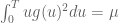 , but I believe the RHS should be
  .
.
24 November, 2013 at 6:02 am
Eytan Paldi
Thanks for the explanation!
25 November, 2013 at 2:53 pm
James Maynard
Just to confirm: Everything that Pace says is correct. Both of these are typos in the paper – sorry for the confusion this caused.
If anyone happens to spot similar typos I’d quite like to hear – either emailing me or mentioning on here would be appreciated!
24 November, 2013 at 6:49 pm
Terence Tao
I can now modify the Cauchy-Schwarz argument to prove the clean upper bound
which saves a or so from the previous bound.
The key estimate is
Assuming this estimate, we may integrate in to conclude that
which symmetrises to
giving (1).
It remains to prove (2). By Cauchy-Schwarz, it suffices to show that
But writing , the left-hand side evaluates to
as required.
This also suggests that extremal F behave like multiples of in the
  variable for typical fixed choices of
  .
.
In the converse direction, I have an asymptotic bound
for sufficiently large k. Using the notation of the previous post, we have the lower bound
whenever is supported on
 ![[0,T]](https://s0.wp.com/latex.php?latex=%5B0%2CT%5D&bg=ffffff&fg=545454&s=0&c=20201002) ,
,  , and
, and  are independent random variables on [0,T] with density
  . We select the function
with , and
, and  for some
  to be chosen later. We have
and
and so
Observe that the random variables have mean
The variance may be bounded crudely by
Thus the random variable has mean at most
  and variance
  , with each variable bounded in magnitude by
  . By Hoefding’s inequality, this implies that
  is at most
  with probability at most
  for some absolute constant
  . If we set
  for a sufficiently large absolute constant
  , we thus have
and thus
as claimed.
Hoeffding’s bound is proven by the exponential moment method, which more generally gives the bound
for any , which is a somewhat complicated, but feasible-looking, optimisation problem in A, T, s. (Roughly speaking, one expects to take A close to
  , T a bit smaller than
  , and
, and  roughly of the order of
  .)
.)
25 November, 2013 at 5:14 am
Eytan Paldi
As an interesting application of this upper bound, we have
1. , so under EH the current method is limited to
 .
.
2. , so Under EH[1/2] the current method is limited to
  .
.
25 November, 2013 at 8:49 am
Aubrey de Grey
Or 42 under the polymath8a results, yes? (I believe the confirmed and tentative versions both give this value.) Or am I overinterpreting earlier posts concerning the derivability of M from varpi?
27 November, 2013 at 2:09 pm
Eytan Paldi
Unfortunately, the particular above (used for the derivation of the upper bound) is not in
  (since the integration of
  with respect to
  gives
gives  – which is not integrable over
  ) – so this
  can’t be used as a basis function for lower bounds evaluation.
It should be remarked that – since it has only logarithmic singularity.
7 December, 2013 at 9:47 am
Eytan Paldi
For the upper bound is
  , while from (7.19) in Maynard’s paper
  – showing that the upper bound is surprisingly good even for
  .
.
14 December, 2014 at 7:28 pm
Eytan Paldi
It seems that there is an error in the above derivation of the lower bound since (not
(not  as in the above derivation!)
[Corrected, thanks – there was a similar factor missing in the bound which cancels out the error. -T.]
1 February, 2015 at 7:44 pm
Eytan Paldi
There is another error in the lower bound derivation: for the probability estimate – which is clearly too crude!
 while the (much smaller!) numerator is only
  .
.
It seems that Hoeffding’s inequality (which is independent of the variance) gives
The problem in using this inequality is that the denominator in the exponent is
Fortunately, by using the above variance estimate, it follows from Bennett’s inequality (or even from Bernstein’s inequality) the probability estimate which implies the (slightly weaker) lower bound
30 December, 2014 at 3:25 pm
Eytan Paldi
For the last lower bound on , it is easy to verify that the lower bound is maximized by (temporarily) fixing
  and maximizing the integral
  over
over  under the two (integral) constraints that
  and
and  are fixed. It is easy to show that the optimal function
  has the form
  for some
  .
. (needed for the lower bound) are simple elementary functions of
  – enabling simpler optimization of the lower bound over the parameters
  .
. , it seems that the paremeters
  can be reparametrized by


Fortunately, the resulting integrals representing
For large
Where are the new parameters.
(Unfortunately, it seems that asymptotically we still get the above lower bound implied by Hoeffding inequality.)
24 November, 2013 at 9:56 pm
xfxie
Seems k0 can drop some, assuming the implementation is correct.
With :
:  =339
=339
Without using the inequalities:
  =385
=385
25 November, 2013 at 10:07 am
Terence Tao
Two small thoughts:
1. The Cauchy-Schwarz argument giving upper bounds on might more generally be able to give upper bounds for the quantity
for any Selberg sieve
regardless of the choice of coefficients , assuming that the error terms are manageable (which presumably means something like
  where
where  is the level of distribution) and also some mild size conditions on the coefficients (e.g. all of size
  ). Upper bounds are of course less directly satisfying than lower bounds (particularly for the purposes of advancing the “world records” table) but would help give a picture of what more one can expect to squeeze out of these methods. (And we also have some possible ways to evade these upper bounds, e.g. by utilising the two-point correlations
  as discussed previously; one could also hope to use other sieves than the Selberg sieve, though I don’t see at present what alternatives would be viable.)
2. As mentioned in Maynard’s paper, the method here would also allow one to produce small gaps in other sets than the primes, as long as one had a non-trivial level of distribution . For instance, if one replaced primes by semiprimes (products of exactly two primes) Goldston-Graham-Pintz-Yildirim obtained the bounds
  and
and 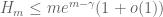 unconditionally. These bounds are already quite good (semiprimes are significantly denser than primes, which is why the results here are better than those for primes) but perhaps there is further room for improvement.
25 November, 2013 at 10:48 am
Terence Tao
Just did a quick calculation: using Maynard’s sieve (with T equal to, say, ) the quantity
  looks to be roughly on the order of
  (compared to
  in the case of primes), by counting products of two primes each of size at least
  . (For semiprimes with smaller factors than this, the sieve weight
  becomes smaller.) So this would give something like
  for semiprimes, and more generally
  for products of exactly r primes (with implied constants depending on r).
Actually, in many ways, the numerology for our current problem with primes is very similar to the GGPY numerology for semiprimes.
25 November, 2013 at 8:06 pm
Terence Tao
Looks like the Cauchy-Schwarz argument does indeed block the Selberg sieve from doing much better than primes in a k-tuple, assuming that the weights are fairly uniform in magnitude, which among other things, allows one to discard the small fraction of weights in which the heuristic
  mentioned in Section 6 of Maynard’s paper fails. The analogue of the ratio
  is then (in the notation of the paper)
Cauchy-Schwarz then gives
for any (using the fact that
  is constrained to be coprime to
  ); using this and summing in
  (using the constraint
  ) shows that the ratio is of size
  , which for bounded choices of A gives a bound of
  . If one works this argument more carefully we get the same upper bounds that we do for the integral variational problem
  .
.
There is a potential loophole in using sieve weights that focus on those moduli r with a unusually large number of prime factors (so that are no longer close to each other), but this is a very sparse set of moduli, to the point where the error terms in the sieve analysis now overwhelm the main terms. Also, intuitively one should not be able to get a good sieve by using only a sparse set of the available moduli.
To me, this suggests that the main remaining hope for breaking the logarithmic barrier is to work with a wider class of sieves than the Selberg sieve. In principle there are a lot of other possible sieves to use (e.g. beta sieve or other combinatorial sieves), but numerically these sieves tend to underperform the Selberg sieve for these sorts of problems (enveloping the primes in a sieve weighted on almost primes in order to make the density of the primes as large as possible). It’s tempting to try to perturb the Selberg sieve in some combinatorial fashion, but the trick is to keep the sieve non-negative (which is crucial in our argument, unless one can somehow get excellent control on the negative portion of the sieve); once one leaves the Selberg sieve form this becomes quite non-trivial.
26 November, 2013 at 3:08 am
Eytan Paldi
Perhaps there is some generalization to a sieve combining translates of several admissible tuples.
26 November, 2013 at 11:06 am
Terence Tao
I’m now leaning towards the view that any replacement for the Selberg sieve will also encounter a logarithmic type barrier, in that the density
  is unlikely to be much higher than
  . Actually it is rather miraculous that we get the logarithmic gain at all, a naive heuristic computation (which I give below) suggests that
  should be the threshold.
To motivate things, suppose we start with a one-dimensional sieve , where
  are some coefficients for
  up to some height
  . In the Selberg sieve case this divisor sum is the square of some other divisor sum
  to ensure non-negativity, but we will not assume here that the sieve is of Selberg type.
The primality density of such a sieve cannot be much larger than
  . This is because all
  -rough numbers (numbers with no prime factor less than
  ) are assigned the same value by the sieve
  , and by the asymptotics for the Dickman-de Bruijn function, the primes in
 ![[x,2x]](https://s0.wp.com/latex.php?latex=%5Bx%2C2x%5D&bg=ffffff&fg=545454&s=0&c=20201002) form a proportion of about
form a proportion of about  of all the
  -rough numbers in
 ![[x,2x]](https://s0.wp.com/latex.php?latex=%5Bx%2C2x%5D&bg=ffffff&fg=545454&s=0&c=20201002) .
.
Now we look at a multidimensional sieve , where again we do not assume the sieve to be of Selberg type, but we impose a restriction of the shape
  since we are unlikely to control the sieve error terms without such a hypothesis, even assuming the strongest Elliott-Halberstam type conjectures. Heuristically, this limits each of the
  to be typically of size
  , and then the one-dimensional argument suggests that the primality density
  should not be much larger than
  for each
  .
.
Now the Maynard sieve does do a bit better than this, because each factor is allowed to be a bit higher than
  on occasion (there is a weight roughly of the shape
  in the sieve), since one can rely on concentration of measure (or the law of large numbers, if you wish) to keep the product
  of a reasonable size
  . This occasional use of higher moduli seems to just barely be sufficient to diminish the sieve
  on some of the other
  -rough numbers than the primes to boost the prime density from
  to
to  . But it seems unlikely that a clever choice of sieve weights could do much better than this.
26 November, 2013 at 12:51 pm
James Maynard
Do you have a heuristic which explains the gain in the log, without looking too much at the sieve functions themselves?
I ask because I’d been working under the same heuristic that you mention above, and it surprised me that the modified weights were able to win by a full factor of a log. I don’t have any good heuristic explanation as to how one might be able to `see’ that these weights do this well a priori. Obviously, although logs are critical in the small-gaps argument, they are very small in comparison to , and so we shouldn’t necessarily be surprised a heuristic breaks down at this level of accuracy.
That said, I liked this heuristic because it seemed to work well with similar problems. It seems to explain quite naturally the results of GGPY/Thorne on small gaps between numbers with prime factors, results on sifting limits and results on the number of prime factors of
  . (Some of these are more `robust’ to a log factor than others). The `superiority’ of the Selberg sieve over other sieves for larger
  seemed to me just that the implied constants in the
  -terms were better.
26 November, 2013 at 9:17 pm
Terence Tao
Unfortunately I don’t have much of an explanation for this – at a formal level it shares a lot of similarities with the logarithmic divergences that show up in the endpoint Sobolev inequalities in harmonic analysis, in that one gets contributions from logarithmically many dyadic scales (which, in this case, would be something like the contribution of moduli between and
and  for
for  ) but the way in which these scales interact seems rather specific to the Selberg sieve, and it is possible that some other sieve might give a different power of log (or more likely, no logarithmic gain at all).
25 November, 2013 at 11:55 am
Aubrey de Grey
Asking the converse question: is there any N for which there are already known to be infinitely many x such that both x and x+2 are products of exactly N primes? If not, is it plausible that Maynard’s methods can be used to identify such an N? (Or if so, to reduce the known N?)
25 November, 2013 at 12:09 pm
Terence Tao
No, this is blocked by the parity problem. Given any sieve candidate , we expect
  and
and  to be negligible (this is part of the “Mobius pseudorandomness heuristic”), which basically means that if
  is drawn at random from the
  distribution, then
  has a probability
  of having an even number of factors, and
  of having an odd number of factors. Similarly for
  . The upshot of this is that one cannot use purely sieve-theoretic methods to prescribe the parity of the number of prime factors of both
  and
and  . But it turns out (as worked out by Bombieri) that on EH, one can basically do anything that does not run into this parity obstruction; for instance one can find infinitely many prime n such that n+2 is the product of either 2013 or 2014 primes. (This should be discussed in Friedlander-Iwaniec’s “Opera del Cribro”, though I don’t have this reference handy at present.)
Breaking the parity barrier for twins would be an absolutely huge breakthrough, even if conditional on Elliott-Halberstam. But it’s going to take a radically new idea; it’s not just a matter of tweaking the sieves.
25 November, 2013 at 11:21 pm
Anonymous
I was wondering if you could elaborate on the intuition for why it will take a radically new idea (similarly, I think I remember you saying that proving or disproving $P versus NP$ will require a new idea. how do you know?) Is it just that a lot of people have tried to solve these problems using many different techniques and failed or is it something else? Thanks.
26 November, 2013 at 9:13 am
Terence Tao
I discuss the parity problem further in my old blog post https://terrytao.wordpress.com/2007/06/05/open-question-the-parity-problem-in-sieve-theory/
27 November, 2013 at 12:00 am
Anonymous
Thanks.
25 November, 2013 at 12:43 pm
Pace Nielsen
Three days ago I started running some computations. Here are the results. Throughout, I will be assuming EH.
————————–
Take . Let
. Let  be an arbitrary polynomial function of total degree
  , which is symmetric in
  and in
  separately. Working over the original simplex
  of Maynard, set
Using a numerical optimizer (so results are not necessarily optimal, but should be close), we get:
For ,
,  .
. ,
,  .
.
For
It is not difficult to increase a little more. Probably up to
  is feasible.
————————–
Take . Let
. Let  be an arbitrary polynomial function of total degree
  , which is symmetric in the variables. Working over the original simplex
  of Maynard, and again using a numerical optimizer, we get:
For ,
,  .
. ,
,  .
. ,
,  .
.
For
For
This is already very close to the upper bound of recently discovered by Terry.
————————-
I then tried to do the case for the new simplex
  , but the numerics give weird answers. For instance, when
  , we get
  . The reason I didn’t post these computations earlier is that I’ve been trying to figure our where my error is. After two days I still have not been able to track down my error. I wrote up a LaTeX document explaining the computation, and I’m willing to email it (and the mathematica file) to anyone who is interested.
25 November, 2013 at 2:34 pm
James Maynard
I reran the computations I alluded to at the beginning of the previous post.
My calculations agree with yours for the original simplex (I get the slightly better bound
 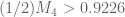 when
when  .)
.)
This is for , using the enlarged simplex
  . As you have done, I’m taking
  to be an arbitrary symmetric polynomial of degree
  on
on  , and then I’m using the linear-programming method from my paper to calculate the eigenvector which corresponds to the optimal choice of coefficients of
  .
.
I then get the bounds


This was my reason for saying using the enlarged simplex gets `about half way’ to obtaining gaps of size 8: we’ve improved from a lower bound of about 0.92 to about 0.96, and we want to get it to 1.
It appears that the convergence as increases is for the enlarged simplex is noticeably slower than for the original simplex.
I can give more details of how I did the calculations if interested.
25 November, 2013 at 4:03 pm
Pace Nielsen
When I figure out where my computational error is, now I’ll know what numerics to look for. Thank you!
P.S. The reason I didn’t send those typos I mentioned above to you, is that I’m reading through your paper with Roger Baker (here at BYU) and he is compiling a list of the typos we run across. He will be sending that to you, probably in a couple of weeks.
25 November, 2013 at 7:35 pm
James Maynard
Oops, there was a small typo in my program. The corrected bounds I get are


 seems good.
and the convergence with
Summary of my calculation:
 ,
, is symmetric, then
  is symmetric in
  . This means the region with
  will contribute
  of the total. In this region, it is straightforward to put exact limits on each integration variable. We get

 . Again, these are quadratic forms in the coefficients of
  , and so we can find the optimal choice of
  of given degree by calculating the largest eigenvalue of a matrix.
we can notice that if
We also get a similar expression for
26 November, 2013 at 2:14 am
Bogdan
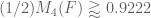
I am a bit confused: the upper bound of 0.924 is reported in post for 25 November, 2013 at 5:14 am, and the conclusion was that “so under EH the current method is limited to k_0=5”, and now you get the lower bound of 0.9689! Is this because of “using the enlarged simplex”?
26 November, 2013 at 11:24 am
James Maynard
Bogdan: Yes, the upper bound of 0.924 was for functions whose support was restricted to the smaller simplex . By comparison, we are getting a lower bound of 0.922 in this case, so these seem to be in good agreement.
If we use a modification of the original method (such as extending the support to the slightly large simplex or incorporating the
  terms) then this upper bound no longer applies. In particular, the lower bound of 0.96 using the larger simplex isn’t in contradiction to the earlier bound.
26 November, 2013 at 5:29 pm
Eytan Paldi
The fast convergence (using polynomials) indicates the (possible) existence of a smooth maximizer.
25 November, 2013 at 3:23 pm
Anonymous
Comments (from a non-mathematician who is interested in mathematics):
In Maynard’s paper, it is stated that , but in the post, it is stated that
  .
.
25 November, 2013 at 4:28 pm
Terence Tao
The bound is unconditional, but the improved bound
  is available if one assumes the Elliott-Halberstam conjecture; this isn’t explicitly stated in Maynard’s paper but it follows easily from the methods of the paper (so if James is revising the paper anyway, one may as well add in that remark).
25 November, 2013 at 3:52 pm
Anonymous
@Maynard:
* The subscript “ ” should be “
 ”.
”.
* When typing maps, one should use “\colon” instead of “:” in order to get the correct spacing aroung the colon.
(Typographical comments, valid throughout the paper.)
26 November, 2013 at 8:28 am
Aubrey de Grey
I’m wondering whether it is possible (or desirable) to reformulate the progress being made here on M_k in a manner that more closely resembles prior work, in particular Polymath8a. Taking things down to their barest essentials, I gather that we can informally say that Maynard and polymath8b have improved the k for which DHL[k,m+1] is implied by EH[theta] (but see below) from an exponentially decreasing function of (theta – m/2) (i.e. GPY) to something on the order of e^(2m/theta). I appreciate that there are good mathematical reasons for working centrally with the quantity M_k, but it’s not clear to me whether the evolving bounds on M as a function of k can be “inverted” to give bounds on k as a direct function of m and theta. If that were possible, I think that for expository purposes it would be of great interest.
Also, I have a somewhat similar question relating to polymath8a. Is it possible to state an explicit version of EH[theta] (let’s call it EH’[theta]) that is implied (up to a value of theta that is a function of i. varpi and delta) by MPZ(i)[varpi,delta], and that also suffices to imply DHL[k,m+1] for sufficiently large k? If that were possible, it seems like it would constitute a nicely clean way, again for expository purposes, to separate the progress in reducing delta from the progress in reducing k for a given theta (and m). Can someone please clarify this?
26 November, 2013 at 8:43 am
Terence Tao
The various upper and lower bounds on Maynard’s sieve all correspond to asymptotics of the form![DHL[ k, (\frac{\theta}{2} + o(1)) \log k ]](https://s0.wp.com/latex.php?latex=DHL%5B+k%2C+%28%5Cfrac%7B%5Ctheta%7D%7B2%7D+%2B+o%281%29%29+%5Clog+k+%5D&bg=ffffff&fg=545454&s=0&c=20201002) for large
for large  , which in particular implies
  for large
  ; the only difference between them lies in the precise nature of the o(1) error term. Once the bounds stabilise, one can of course work these things out more accurately.
The Bombieri-Vinogradov theorem already implies![DHL[k,m+1]](https://s0.wp.com/latex.php?latex=DHL%5Bk%2Cm%2B1%5D&bg=ffffff&fg=545454&s=0&c=20201002) for sufficiently large k, and is a known theorem and is thus implied by any MPZ type statement. We do have some implications that do a little better than this by exploiting an MPZ hypothesis, by using a cutoff function F for Maynard’s sieve that is supported in an appropriate cube; again, the asymptotics for large m or large k are as above (in particular, the role of delta is asymptotically negligible), but the situation seems to be more complicated in the non-asymptotic regime, e.g. when m=1 or m=2.
for sufficiently large k, and is a known theorem and is thus implied by any MPZ type statement. We do have some implications that do a little better than this by exploiting an MPZ hypothesis, by using a cutoff function F for Maynard’s sieve that is supported in an appropriate cube; again, the asymptotics for large m or large k are as above (in particular, the role of delta is asymptotically negligible), but the situation seems to be more complicated in the non-asymptotic regime, e.g. when m=1 or m=2.
26 November, 2013 at 9:36 am
Aubrey de Grey
Thanks! On the first point, absolutely – I just couldn’t exclude the possibility that this inversion might be so easy that there would be no reason to defer it. On the second point, sure, I was of course referring to an EH’ that would do the job for theta > 1/2; however I was mainly referring simply to the pre-Maynard universe and wondering whether this kind of condensation of i, varpi and delta down to a single parameter theta is possible at all.
26 November, 2013 at 11:33 am
Aubrey de Grey
In other words, when I wrote “for sufficiently large k” I should have written “for the same k that MPZ(i)[varpi,delta] itself does”.
26 November, 2013 at 1:13 pm
Terence Tao
A minor (and standard) remark: the Selberg sieve can be rewritten as
where are as in Maynard’s paper and
  are the Ramanujan sums
(restricting to squarefree ); this is basically equation (5.8) of Maynard’s paper after some rearranging.
The functions behave approximately like independent random variables as
  vary, which heuristically explains why the mean value of
  is basically
 in terms of the
  (Lemma 5.2 of Maynard’s paper). I wasn’t able to use this representation of the Selberg sieve for much else, though.
and can also give heuristic justification for the asymptotic for
26 November, 2013 at 2:51 pm
Anonymous
Typographical comment to Terry: If you use $\dots$ instead of $\ldots$, LaTeX will take case of correct placement of the dots; they shouldn’t always be lowered to the base of the line.
26 November, 2013 at 3:34 pm
Eytan Paldi
In the definition of , the functions
  need only to be in
 (i.e. not necessarily bounded.)
26 November, 2013 at 5:10 pm
Pace Nielsen
In the spirit of “A poor man’s improvement on Zhang’s result”, I was playing around with Maynards mathematica notebook. I found that increasing “p[5]” to “p[6]” (and increasing the number of variables to 56, and precomputing polynomials up to degree 13) allows one to push . This was confirmed by Maynard. [It appears that no further gain is made in such an easy manner by just increasing the degree further.]
Obviously, further improvements are available if we incorporate some of the higher order power-symmetric polynomials like P_3.
26 November, 2013 at 9:57 pm
Sniffnoy
102 or 103? It says 102 here but 103 on the wiki and I’m wondering whether that is a typo here or a copying error there (the H value listed there is for 103).
[Corrected, thanks – T.]
27 November, 2013 at 8:44 am
Terence Tao
Here is a possible way to generalise the Selberg sieve. We’ll use the “multiimensional GPY” formulation
for the sieve, where F is a smooth function supported on the simplex (or the enlarged simplex). We can square this out as
One can then consider the more general sieve
for some smooth function supported on the product of two simplices. This function obeys similar asymptotics to the original sieve (this can be seen for instance by using Stone-Weierstrass to approximate
  by a finite linear combination of tensor products, or else by direct computation); for instance one has
if the denominator is non-zero, where the subscripts on F denote differentiation in one or more of the variables . The main problem is that without further hypotheses on
  , the sieve weight
  is not necessarily non-negative, which is a crucial property in the argument. In the case that
  is positive semidefinite (viewed as a “matrix” or “quadratic form” on the simplex), one obtains the non-negativity; but in this case one can diagonalise F into a non-negative combination of Selberg sieves, which cannot give better ratios than a pure Selberg sieve. However, it may be possible to have
  non-negative even without
  being positive semidefinite, leading to a genuinely more general class of sieve. The positivity requirement is a bit complicated though, even in the base case k=1; a typical condition is
whenever . This condition demonstrates the non-negativity of
  for products of two primes; one needs similar conditions for products of
  primes for any bounded r, and this should suffice (note that these sieves are concentrated on numbers with only a bounded number of prime factors).
 , but hopefully they are a bit weaker, allowing for more test functions
  to play with.
These conditions are implied by positive semi-definiteness of
27 November, 2013 at 3:22 pm
Terence Tao
A cute inequality related to the above considerations: for any smooth function![F: [0,1] \to {\bf R}](https://s0.wp.com/latex.php?latex=F%3A+%5B0%2C1%5D+%5Cto+%7B%5Cbf+R%7D&bg=ffffff&fg=545454&s=0&c=20201002) , one has
, one has
where and
and  is the difference operator
  . Thus for instance
The sieve theoretic interpretation is that the right-hand side is an appropriately normalised version of if
if  , and the left-hand side is the contribution to
  coming from products of exactly
  primes for
  . For sufficiently smooth functions F (e.g. finite linear combinations of exponentials), the inequality is in fact an identity, as can be seen by a rather fun computation. The claim can also be proven from the recursive distributional identity
for , where
  is the nonlinear operator
27 November, 2013 at 5:57 pm
James Maynard
A couple of calculations regarding attempts to modify the case to obtain gaps of size 8:
Using the enlarged simplex, I get that (and I would expect this to be close to the truth). This means that the `probability’ that one of the elements of a 5-tuple is prime is
  . If we assume independence, then we would expect the probability that both
  and
and  are prime to be
  (since we don’t expect to be able to get an asymptotic for this quantity, in reality we have to satisfy ourselves with an upper bound, which would be worse than this). This means that the modification of taking away the contribution form the times when
  and
and  are simultaneously prime would (in the most optimistic scenario) leave us with a total of
  . This means we need at least one new idea to improve the situation. We'd need a lower bound on
  which is certainly greater than
  for this modification to get us over the edge.
I also tested the upper bound to see how it fared numerically. My calculations should be treated as very provisional, since I haven't checked them properly. In the scenario above, I find that taking a suitable polynomial for , we get a lower bound for the modified version of
  which gives
  . This compares well with the most optimistic bound of
  from above. This also corresponds to an upper bound for
  of size
  , which again is close to the guessed asymptotic value of
  .
.
Since these bounds performed quite well, it is maybe reasonable to expect us to get decent upper bounds when we are considering or similar. I don't know how we would evaluate the integrals that arise, however.
27 November, 2013 at 6:40 pm
Terence Tao
Thanks for these calculations! Due to the parity problem, I expect that any upper bound we obtain on is going to be off by a factor of at least 2 from the truth (so in this case, it would be like
  rather than
  ). This isn’t consistent with the
  number that you are provisionally reporting, but perhaps the numerology for the
  optimiser is a bit different from that for the
  optimiser. For instance, it may be advantageous to break symmetry a bit and work with polynomials F that behave differently in the
  variables than in the
  , lowering the probability that n is prime and n+12 is prime (in order to also lower the probability that n,n+12 are both prime) while also raising the probability that n+2,n+6,n+8 are prime.
0.987 is tantalisingly close to 1, so there is still hope :) Certainly things should look better for larger k. One relatively cheap thing to try is just to take the best polynomial we have for and compute the upper bounds on
  (note though that if we retreat from EH to Bombieri-Vinogradov, some of the 1/2 factors in the previous formula for this quantity degrade to 1/4).
27 November, 2013 at 6:52 pm
Terence Tao
A small observation: somewhat frustratingly, the Zhang/Maynard methods do not quite seem to be able to establish Goldbach’s conjecture up to bounded error (i.e. all sufficiently large numbers are within O(1) of the sum of two primes). But one can “split the difference” between bounds on H and establishing Goldbach conjecture with bounded error. For instance, assuming Elliott-Halberstam, one can show that at least one of the following statements hold:
1. (thus improving over the current bound of
  ); or
); or
2. Every sufficiently large even number lies within 6 of a sum of two primes.
To prove this, let N be a large multiple of 6, and consider the tuple n, n+2, n+6, N-n, N-n-2. One can check that this tuple is admissible in the sense that for every prime p, there is an n such that all five elements of the tuple are coprime to p. A slight modification of the proof of DHL[5,2] then shows that there lots of n for which at least two of the five elements of this tuple are prime; either these two elements are within 6 of each other, or sum to a number between N-2 and N+6.
If we can ever get DHL[4,2] (or more precisely, a variant of this assertion for the tuple n, n+2, N-n, N-n-2), we get a more appealing dichotomy of this type: either the twin prime conjecture is true, or every sufficiently multiple of six lies within 2 of a sum of two primes.
28 November, 2013 at 8:54 am
Aubrey de Grey
Wow! This immediately raises two questions that would surely be of wide interest:
1) For k=5, can one split the difference unevenly, i.e. lower the value 6 in one statement at the expense of using a number larger than 6 in the other? If so, how unevenly – all the way to TP or Goldbach?
2) Can analogous statements be made for larger k? In particular, for k large enough to require only BV (or MPZ) rather than EH?
28 November, 2013 at 11:19 am
Aubrey de Grey
In fact, much better would be to unify the above questions in the obvious way, as follows:
If we denote by “GBE[n]” (Goldbach up to bounded error n – is there an established name for this conjecture?) the assertion that all even numbers are within n of an even sum of two primes (I’m omitting “sufficiently large” here only because I presume that “sufficiently” can easily be shown in this context to be within the range for which GC itself has already been computationally verified – apologies if that’s not true), then for which [a,b,c] can we say that DHL[a,2] implies DHL[b,2] or GBE[c] ? Terry’s observations constitute this statement for [a,b,c] = [5,3,6] and [4,2,4]. How far can the allowed values be broadened?
27 November, 2013 at 9:33 pm
Anonymous
I feel that Goldbach’s conjecture / twin primes conjecture are very close to be proved.
All originated from Zhang’s work!
27 November, 2013 at 10:17 pm
Gil Kalai
I am curious about is the following. Consider a random subset of primes (taking every prime with probability p, independently, and say p=1/2). Now consider only integers involving these primes. I think that it is known that this system of “integers” satisfies (almost surely) PNT but not at all RH. We can consider for such systems the properties BV (Bombieri Vinogradov), or more generally EH(θ) and the quantities . For such systems does BV typically hold? or it is rare like RH. Is Meynard’s implication applies in this generality? Nicely, here we can hope even for infinite consecutive primes.
28 November, 2013 at 8:26 am
Terence Tao
Strictly speaking, if only takes half of the primes, then the remaining integers is a very sparse set – about elements up to
  – which makes all the numerology very different from that of the full primes.
You may be thinking instead of the Beurling integers, in which the primes are replaced by some other set of positive reals with the same asymptotic density properties. These integers enjoy many of the same “multiplicative number theory” properties as the usual integers (e.g. the prime number theorem), but one usually loses all of the “additive number theory” properties, basically because the Beurling integers are not translation-invariant: if n is a Beurling integer, then n+2 usually isn’t, and so asking for things like twin Beurling primes is not really a natural question; similarly for questions about distributions of Beurling primes in residue classes (Bombieri-Vinogradov, EH, etc.) (unless one also somehow creates a theory of “Beurling Dirichlet characters” to go with the Beurling primes, but I do not know how to make this work for anything that isn’t already coming from a number field).
28 November, 2013 at 10:32 am
Gil Kalai
Terry, how can it be if you leave half the primes alive?
28 November, 2013 at 10:51 am
Terence Tao
Oops, I miscalculated; the density is now rather than
  , so I drop my previous objection to the question :). (My error was thinking that the average number of divisors of n would remain comparable to
  , when instead it drops to
  .) The main technical difficulty now is with counting such quantities as the number of integers n less than x such that n and n+2 are both divisible by the surviving primes; offhand I don’t see a promising technique to answer this question (as well as more general questions in which several shifts of n are involved, and some congruence class conditions on n are also imposed) but it looks like an interesting problem.
28 November, 2013 at 11:21 am
Gil Kalai
Indeed, I was thinking about Beurling integers, and my questions can be asked about them but I wanted a very very specific model which will make computations easier. I think that it is not that easy to work with general Beurling primes and finding a concrete stochastic models (like random graphs, sort of) may be more fruitful.
If we want to keep the density of primes on the nose we can possibly still take p_n with independent but not identical probabilities not to corrupt asymptotic density properties, or do some other “correction”, but perhaps taking half the primes is also of interest.
All the questions I asked refer only to the relative ordering of the Beurling integers and *not* to their additive properties. So “twin primes” refers to two Beurling primes with a single composite Beurling integer in between. And “consequtive primes” refers to two Beurling primes without any composite Beurling integer in between (Alas, we don’t have them often in the usual case.) I think that PNT, RH, BV (Bombieri Vinogradov), or more generally EH(θ), and (in the *ordinal*, not *additive* sense) continue to make sense (perhaps even more than one sense) for Beurling primes and it is interesting to see if Meynard implication extends, but it looks to me that considering a stochastic model based on the primes will make the issue more tractable (and perhaps useful).
28 November, 2013 at 12:28 pm
James Maynard
If I understand your question correctly, then I would have thought for such a system you would get (almost surely) for this subset of the primes, whenever
  holds for the primes themselves. (And so bounded gaps with
  primes).
If is the number of chosen primes in the residue class
  which are at most
  , then
  is distributed as a binomial random variable
  . Therefore, we should get, for some constant
In particular, over all for which
  we have almost surely
  . (There are
  such pairs
  , and we take
  above). The errors from these
  -terms are negligible. The errors from those pairs
  for which `
 ‘ does not hold, and the errors
  can be bounded by regular
  for all primes.
28 November, 2013 at 1:52 pm
Terence Tao
I agree that this form of![EH[\theta]](https://s0.wp.com/latex.php?latex=EH%5B%5Ctheta%5D&bg=ffffff&fg=545454&s=0&c=20201002) will hold almost surely, but I think for applications to bounded gaps between these Beurling-type integers one needs a significantly stronger version of
will hold almost surely, but I think for applications to bounded gaps between these Beurling-type integers one needs a significantly stronger version of ![EH[\theta]](https://s0.wp.com/latex.php?latex=EH%5B%5Ctheta%5D&bg=ffffff&fg=545454&s=0&c=20201002) in which one not only counts those
in which one not only counts those  for which
  is a Beurling prime, but also
  is a Beurling integer for the other elements
  in the tuple.
Actually, never mind bounded gaps between Beurling primes: bounded gaps between Beurling integers is already somewhat non-trivial problem, particularly if one wants the correct asymptotic for how often this occurs; this is probably the main obstacle to extending the various results for gaps between primes to this Beurling setting.
28 November, 2013 at 3:16 pm
James Maynard
Can you not use the sieve as before, comparing to just the constant function 1 (supported on all integers, Beurling-type or not)?
Since you have for these primes, you should be able to calculate an asymptotic for the sieve weighted by these terms (which will be 1/2 of what we get for primes). Since
  tends to infinity, I would have thought we should then get
  primes in a
  -tuple whenever we would have got
  primes before.
28 November, 2013 at 4:24 pm
Terence Tao
Well, if one uses the existing sieve without any modification, the density
  will only be of the order of
  , which is too sparse to pick up more than one prime in the tuple. Things are presumably better if one replaces
  by
by  , but then one needs asymptotics for things like
  , which is presumably doable but requires some calculation. (It is vaguely reminiscent of the Titchmarsh-type divisor problem of finding integers n, n+h with specified divisor function.)
28 November, 2013 at 1:50 pm
Terence Tao
A new paper on the arXiv by William D. Banks, Tristan Freiberg, and Caroline L. Turnage-Butterbaugh: “Consecutive primes in tuples“. Basically they show that Maynard’s result can be boosted to guarantee that the m primes involved are consecutive, although they have to increase k somewhat (to be double exponential in m rather than single exponential) to do this. (It may be, though, that one can avoid this by computing asymptotics for for h not in the tuple, much as in the original GPY paper, or by using the ideas of Pintz as is done for instance in http://arxiv.org/abs/1305.6289 .)
28 November, 2013 at 2:59 pm
Eytan Paldi
Perhaps this new type of (for consecutive primes) may be studied here as well.
30 November, 2013 at 7:38 pm
Kalpesh Muchhal
Hi, Corollary 3 of the Banks-Freiberg-TB paper shows that consecutive primes can be part of an AP, while the Green-Tao theorem shows that primes can be consecutive terms of an AP. Can these results be somehow combined to prove consecutive primes can be consecutive terms of an AP infinitely often?
30 November, 2013 at 9:39 pm
Terence Tao
Unfortunately, the primes that we can capture in short intervals are so sparse (one roughly has only or so primes in an interval of length H) that it is not presently possible to force them into arithmetic progression. (My arguments with Ben can produce arithmetic progressions of primes in
 ![[x,x+x^{o(1)}]](https://s0.wp.com/latex.php?latex=%5Bx%2Cx%2Bx%5E%7Bo%281%29%7D%5D&bg=ffffff&fg=545454&s=0&c=20201002) – this was explicitly noted in a later paper of myself with Ziegler – and in view of more recent work (particularly that of Conlon, Fox, and Zhao) it is likely that one can narrow this to
– this was explicitly noted in a later paper of myself with Ziegler – and in view of more recent work (particularly that of Conlon, Fox, and Zhao) it is likely that one can narrow this to ![[x,x+\log^{O(1)} x]](https://s0.wp.com/latex.php?latex=%5Bx%2Cx%2B%5Clog%5E%7BO%281%29%7D+x%5D&bg=ffffff&fg=545454&s=0&c=20201002) – but this is still a bit too wide to expect that the primes produced in this fashion will be consecutive.)
– but this is still a bit too wide to expect that the primes produced in this fashion will be consecutive.)
29 November, 2013 at 7:53 am
Andrew Granville
I do not see why one needs to increase k. If the m-prime result is obtained from the k-tuple, {x+0, x+a_2,…, x+a_k} then we can restrict ourselves to a congruence class (for x) so that x+j has a given smallish prime factor p_j for each j<a_k, which is not an a_i. The congruence x=-j mod p_j, combine to mean we can write x = Q n +b (where Q = prod_j a_j). Hence we work instead with the k-tuple Qn+b, Qn+b+a_2,…,Qn+b+a_k
I think that one can apply the main theorem directly to this k-tuple, so it has (single) exponential size in m
29 November, 2013 at 8:08 am
Andrew Granville
Beurling primes do not satisfy RH in general… You should look for the beautiful 2006 paper of Diamond, Montgomery and Vorhauer. In fact they show that one can have a Siegel-type zero (which perhaps explains why these are so hard to deal with in the actual prime case).
There was also some mention, amongst these comments, of probabilistic models… of course the Gauss-Cramer model, where a random number n is “prime” with probability 1/log n, predicts that there are many prime pairs n, n+1, so needs some adjusting to take account of correlations arising from local divisibility. Sound and i showed some years ago that all of the obvious models proposed to make these sort of corrections have serious flaws (see our paper “An arithmetic uncertainty principle”).
29 November, 2013 at 10:32 am
Gil Kalai
More about systems of Beurling primes:
About my initial suggestion to take half the primes at random, since a quarter of all pairs of primes survive anyway it does not look that the implication (if it applies) from BV(Bombieri-Vinogradov) or EH(θ) to bounded gap is useful here.
Regarding Beurling primes in general. I see three issues
1) Does (or when) Meynard implication from EH(θ) (or just BV) to bounded gaps applies to general systems of Beurling primes with the right density.
2) Can you either show it more easily or apply it more easily for stochastic systems based on ordinary primes.
3) If (or when) the implication is correct, can you get something useful from it for the current project (or even just interesting consequences otherwise.)
I don’t know about 1) but let me just assume it.
Regarding 2) for most natural models small gap pair of primes will survive. (maybe for k-tuples for large k interesting things can be said. since their rate of survival decay exponentially.) Another stochastic model that is interesting is to take all primes *with* repetitions and to take every prime with (say) Poisson or exponential distribution of mean 1. (For applying it we may need bounds on gaps between 2 to m, so that we can ignore repeated primes.) (One of the most beautiful and useful ideas in modern statistics is to study sequences by sampling from them with repetitions.)
Regarding 3) there are various things to think about. You can delete for your Beurling system all pair of primes of gaps at most 1000 (say). Now, for what we know on the number of primes involved with a gap at most 1000 is too high for the statement of Bombieri-Vinogradov to remain correct automatically. (But it is interesting if it remains correct.) However, we may try using it as part of an argument showing that there are many primes of gaps 1000 or less: If the density of those is small then when we delete them EH is not harmed and we can apply the reduction again. This is not a complete argument since new pairs of primes with small gaps (with respect to the new system) may emerge.
Since the estimates for k-tuples density are especially week compared to reality this type of hypothetical argument may work for them better.
Another similar suggestion is to choose for our Beurling system a random prime from every second interval of integers of length 1000. This automatically eliminate (additive) gaps below 1000.
(If such considerations can “just” lead to new examples of Beurling primes which violate RH, BV, or EH this would also be nice, of course.)
1 December, 2013 at 5:01 pm
Gil Kalai
On more thought, I don’t see how to formulate the above questions for general Beurling primes without the additive structure.
1 December, 2013 at 10:41 am
Terence Tao
I’m recording how to use multiple dense divisibility to (in principle at least) improve the value of k, although at present we can only effectively calculate the various integrals involved when the function F is basically built from a tensor product , which isn’t the case for our best value 102 for k at m=2, but only for the larger value 339 (for m=2) or 43,134 (for m=3).
To review the situation: under![EH[\theta]](https://s0.wp.com/latex.php?latex=EH%5B%5Ctheta%5D&bg=ffffff&fg=545454&s=0&c=20201002) , we can obtain
, we can obtain ![DHL[k,m+1]](https://s0.wp.com/latex.php?latex=DHL%5Bk%2Cm%2B1%5D&bg=ffffff&fg=545454&s=0&c=20201002) (and hence
(and hence  ) whenever we can find a (bounded measurable) symmetric function
  supported on the simplex
  with
with
and
A good choice for F here is a function of the form
where![g(t) = \frac{1}{1+At} 1_{[0,T]}(t)](https://s0.wp.com/latex.php?latex=g%28t%29+%3D+%5Cfrac%7B1%7D%7B1%2BAt%7D+1_%7B%5B0%2CT%5D%7D%28t%29&bg=ffffff&fg=545454&s=0&c=20201002) for some parameters
for some parameters  (in practice we take
  close to
  and
and  close to
  ), and
  . Hypothesis (1) is automatic, and the left-hand side of (2) can be bounded from below by
where are iid random variables with distribution
  .
.
If one wishes to use![MPZ[\varpi,\delta]](https://s0.wp.com/latex.php?latex=MPZ%5B%5Cvarpi%2C%5Cdelta%5D&bg=ffffff&fg=545454&s=0&c=20201002) as the starting hypothesis instead of
as the starting hypothesis instead of ![EH[\theta]](https://s0.wp.com/latex.php?latex=EH%5B%5Ctheta%5D&bg=ffffff&fg=545454&s=0&c=20201002) , one replaces
, one replaces  by
by  , and one has to add the additional hypothesis that
  is supported in the cube
 ![[0,\tilde \delta]^k](https://s0.wp.com/latex.php?latex=%5B0%2C%5Ctilde+%5Cdelta%5D%5Ek&bg=ffffff&fg=545454&s=0&c=20201002) with
with  . The latter hypothesis is obeyed if
If one uses the stronger hypothesis![MPZ^{(i)}[\varpi,\delta]](https://s0.wp.com/latex.php?latex=MPZ%5E%7B%28i%29%7D%5B%5Cvarpi%2C%5Cdelta%5D&bg=ffffff&fg=545454&s=0&c=20201002) instead, one can relax the support condition on
instead, one can relax the support condition on  to the intersection of the larger cube
 ![[0, \tilde \delta']^k](https://s0.wp.com/latex.php?latex=%5B0%2C+%5Ctilde+%5Cdelta%27%5D%5Ek&bg=ffffff&fg=545454&s=0&c=20201002) and the set of
and the set of  such that
where
and is arbitrary with
  ; this follows from Lemma 4.13 of the Polymath8a paper. This has the effect of relaxing (4) to
at the cost of worsening (3) to
We may optimise by making (4)’ an equality.
Using the exponential moment method, we can lower bound (3′) by
where
and
and s,s’ may be chosen as we please. Thus: we obtain![DHL[k_0,m+1]](https://s0.wp.com/latex.php?latex=DHL%5Bk_0%2Cm%2B1%5D&bg=ffffff&fg=545454&s=0&c=20201002) whenever we can find
whenever we can find  obeying
with given by equality in (4′), with
  . Our best estimate for
 ![MPZ^{(i)}[\varpi,\delta]](https://s0.wp.com/latex.php?latex=MPZ%5E%7B%28i%29%7D%5B%5Cvarpi%2C%5Cdelta%5D&bg=ffffff&fg=545454&s=0&c=20201002) is with
is with  and
and  .
.
1 December, 2013 at 5:04 pm
Eytan Paldi
[Oops, there was a typo in the definition of , now corrected. -T.]
2 December, 2013 at 9:36 am
Eytan Paldi
There is a typo in the last inequality (last line.) [Fixed, thanks – T.]
2 December, 2013 at 9:52 am
Terence Tao
I spent some time this weekend reading up on the beta sieve (and on its role in the proof of Chen’s theorem that there are infinitely many primes p such that p+2 is an almost prime (the product of at most two primes)), in the hope that it could be a viable substitute for the Selberg sieve for this project; in particular, I think it would be a great result if one could find an alternate proof of bounded gaps between primes that did not rely fundamentally on a Selberg-type sieve. Unfortunately, it seems that while just about any of the standard sieves (including the beta sieve) can produce probability distributions for which one has for some small constant c and all i=1,…,k, it seems thus far that only the Selberg sieve can get c larger than 1 (which gives bounded gaps between primes) and to even grow logarithmically in k (which gives bounds on
  for all m). I still do not have a clean conceptual understanding of why the Selberg sieve can do this; I have a vague sense that there is some interplay between the “L^2” nature of the Selberg sieve, and the “L^1” nature of density of primes in that sieve, but my intuition on this is still lacking. For the beta sieve, the best I can do is to multiply together k one-dimensional beta sieves of level
  ; it is not obvious to me how to create a genuinely k-dimensional beta sieve, although this is perhaps worth pursuing. (I was intending to write up some notes on the beta sieve but they would basically duplicate a chapter of “Opera del Cribro”, in particular there are some rather tricky calculations involving delayed difference equations which I have thus far been unable to avoid.)
Incidentally, in “Opera del Cribro” it is noted that one can prove Chen’s theorem using a combination of beta and Selberg sieves if one uses the FI distribution theorems (which roughly speaking give a level of distribution of 4/7 (or in our notation, ) when specialised specifically to the twin prime problem). Roughly speaking, the beta sieve gives a lower bound on the number of numbers
  with
with  prime such that
  has no prime factors less than
  , and the Selberg sieve gives an upper bound on the number of primes
  such that
  is the product of three primes greater than
  , and subtracting the two one gets a positive lower bound for the pairs needed for Chen’s theorem. It may be worth revisiting the proof of the FI distribution theorem and see if it may somehow be combined with some of Zhang’s ideas to get new distribution theorems that are usable for the k-tuple problem and not just the twin prime problem. (I did check to see if one can use the special structure of the coefficients in the error terms in the Zhang/Polymath8a arguments, but these coefficients get eliminated as a by-product of the van der Corput process and other necessary applications of Cauchy-Schwarz, so it is not obvious how to exploit the structure. Though FI, BFI, etc. did somehow manage this…)
3 December, 2013 at 12:04 am
Terence Tao
Here is a side benefit of the multidimensional sieve in Maynard’s paper: it gives a new upper bound on the number of such that
  are all prime, i.e. the number of fully prime k-tuplets. The standard sieves (Selberg sieve, large sieve, beta sieve) all give an upper bound of
  for this quantity for some absolute constant C and sufficiently large x, as can be seen by looking up Friedlander-Iwaniec’s book; here
  is the singular series, thus this bound is basically
  worse than what the prime tuples conjecture predicts. (The large sieve and Selberg sieve give a slightly better value for C here than the beta sieve.) If one inserts in the multidimensional sieve, one can improve this to
  (in fact one gets this bound whenever one sieves k residue classes modulo p for all large primes p from an interval of length x). Basically, the problem is now to minimise the ratio
rather than maximise the ratio
but the two variational problems are comparable in much the same way that the root test and ratio test are comparable in undergraduate analysis.
In the converse direction, if one can find another sieve that gives a bound of for the number of fully prime k-tuplets, then this sieve is likely to also be able to obtain bounded gaps between primes, or to find short intervals with many primes in them.
3 December, 2013 at 7:18 am
Terence Tao
Oops, turns out I made an arithmetic error :(. The sieve in Maynard’s paper actually gives the same bound as existing sieves, and this is the limit of the Selberg sieve method (with
  ,
,  being the level of distribution), basically because the volume of the simplex is
  . As with the root and ratio tests, one only has one direction of the implication: a sieve that can beat the
  bound for the k-tuple problem will also likely give many primes in short intervals, but the converse is not necessarily true.
Still it looks like an interesting problem to get for the k-tuple problem. In the converse direction, the parity problem obstruction suggests a lower bound of
  .
.
3 December, 2013 at 7:29 am
Andre
Is there still a need for your new simplified minimization problem?
4 December, 2013 at 2:26 pm
Anonymous
I was asking, because I think I have found polynomials of degree
  with
with
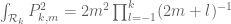
 ,
, .
.
and
which would have given better bounds than the trivial
4 December, 2013 at 10:18 pm
Terence Tao
I should have mentioned that in the simplified variational problem, F has to vanish to sufficiently high order on the boundary of the simplex to be admissible. With that assumption, one obtains from the fundamental theorem of calculus that , and so the Cauchy-Schwarz inequality tells us that the extremum occurs when
  on the simplex (strictly speaking, one has to smoothly truncate this near the boundary of the simplex, but the error incurred from this can be made arbitrarily small), so the infimal value of this ratio is the reciprocal of the volume of the simplex, i.e.
  .
.
4 December, 2013 at 4:13 am
The new Prime gap | On the learning curve...
[…] discussed within the community. Terrance Tao again has this nicely articulated and maintains a polymath page for us. As an onlooker, I am as excited as many others to see this […]
4 December, 2013 at 4:48 pm
Pace Nielsen
I thought I would give a quick update on some recent progress in optimizing the methods described in James’ preprint. (As these ideas are already implicit in James’ paper, I’ve told him he is free to use these bounds in the final version of his paper, so they are not properly part of the polymath8b project, but they still might be of interest to people here.)
As usual, let be fixed. Let
  be a sequence of integers. We say that
  is the signature for the monomial symmetric polynomial
  , and that
  is the degree. The monomial symmetric polynomials form a vector space basis for the space of symmetric polynomials, and James has a good way of integrating these polynomials over
  , with a formula already appearing in his preprint.
So, I wrote a program to search for an optimal solution using such polynomials, up to a given degree. It turns out that there are significant gains over previous computations, and for degree one can get
  and this is optimal for that degree. Increasing the degree further increases
  further, but because of the way I coded the program it runs into RAM issues for
  . [It has problems computing the permutations of the set
  (where
  each occur exactly 11 times.]
To overcome this, I starting doing what James does in his paper, working with polynomials of the form . Taking
  allows one to get down to
  .
.
We are hopeful that eventually these computations will get the optimal , but there is still a lot of optimizing to do. Currently, taking
  , the computation takes about 1 day for a single value of
  .
.
James and I have some ideas about how to fix the RAM issue and so further improvements are forthcoming. [For example, one option is to restrict to signatures for which the number of nonzero terms is at most 10.] Anyone interested in running the Mathematica code on their own computer can email me. (Running it shouldn’t be a problem, but I didn’t make many comments in the code, so it may take a bit of work to understand it.)
4 December, 2013 at 10:33 pm
Terence Tao
Very nice to hear! For comparison, the upper bound shows that k should not be able to go below 50, and for k=64, we have
  (we need
  to win here on Bombieri-Vinogradov). So things are pretty consistent here (and the upper bound is looking remarkably sharp, all things considered – this may suggest some sort of clue as to what the extremising F are behaving like, and possibly to suggest a better theoretical ansatz for F than the one we are currently using (a truncated tensor product) that has only managed to get down to k=339 thus far).
One might hope that the computations get a little bit faster as k drops. Hopefully it becomes small enough that we can begin computing the effect of truncating the simplex a bit to use MPZ (and also to enlarge the simplex to the slightly larger convex body that is available, and perhaps also to try to use the upper bounds on to shave a little bit more off of H).
5 December, 2013 at 4:41 am
Eytan Paldi
For , this implies that under EH the best
  under the current method is in
 ![[51, 64]](https://s0.wp.com/latex.php?latex=%5B51%2C+64%5D&bg=ffffff&fg=545454&s=0&c=20201002) .
.
5 December, 2013 at 7:24 am
Pace Nielsen
Currently, the dependence of the timing of the computation on the value of is minimal–it just changes the coefficients a bit but the number of coefficients is unchanged. Eventually
  would have an effect, by limiting the lengths of signatures, but as I suggested above, we may need to artificially impose a limit on such lengths to make the computations feasible. (And for
  this effect would only naturally start taking place when
  or so.)
I too have thought about whether or not these computations would give us a better idea where to look for the optimal . I’ll try to look for a pattern in the structure of the optimal
  for a given degree as
  increases, and report back if I see anything.
5 December, 2013 at 7:44 am
Aubrey de Grey
Pace, could you post a list of the optimal F you’ve found for each degree up to 10? I think it would be fun for everyone to look for such a pattern.
5 December, 2013 at 12:19 pm
Pace Nielsen
Aubrey,
How would you like the data? Would the coefficients of the monomial symmetric polynomials work for you?
5 December, 2013 at 12:34 pm
Aubrey de Grey
Well, I’m not equipped to make nearly so much use of the data as others here, so I’d prefer to defer to the group as to format. I guess I was assuming that you would essentially emulate equation 7.18 from James’s paper, but please use whatever format seems most convenient and we can all complain as needed :-)
5 December, 2013 at 9:26 am
Eytan Paldi
For a given polynomial , let
, let  . My suggestion is to use
  (for some N) as a new basis (or add them to the current basis.)
4 December, 2013 at 10:36 pm
Childman
Since it may get increasingly computationally intensive to get lower values of k, it may be a good idea to rewrite the optimization code for some kind of grid or distributed computing..
4 December, 2013 at 6:38 pm
Fan
For , we have a bound
  .
.
5 December, 2013 at 12:58 pm
Pace Nielsen
As suggested by Aubrey and Roger Baker here at BYU, I’ve now looked at the coefficients of the maximizing function of a given degree. I have not seen any pattern, but that may be due to a number of different factors. Here is a partial list of the data. For the full list just email me and I’ll send you the file.
Throughout, take (which gives gap sizes of
  , so it would be really nice to reach this point). First, let me list the lower bounds on
  for each degree.
For ,
,  .
. ,
,  .
. ,
,  .
. ,
,  .
. ,
,  .
. ,
,  .
. ,
,  .
. ,
,  .
. ,
,  .
. ,
,  .
.
For
For
For
For
For
For
For
For
For
Any idea if this sequence is converging below 4?
To give the coefficients of , we first need a way to order the signatures. First, to save space we can drop any zeros from the end of a signature, so the signatures correspond to the partitions of the degree. I then order the signatures first according to total degree, and then according to how Mathematica orders the partitions (which is by taking the maximal
  , then the maximal
  etc…).
So, my signatures start out as: .
.
For , the coefficients are
  .
. , the coefficients are
  .
. , the coefficients are
  .
.
For
For
The entries continue to decrease as increases.
5 December, 2013 at 1:00 pm
Pace Nielsen
(Of course, the above was also suggested by Terry.)
When I said that the entries decrease, I meant in absolute value. They continue to change signs.
5 December, 2013 at 1:21 pm
Andre
perhaps with some more digits, the inverse symbolic calculator might help
http://oldweb.cecm.sfu.ca/projects/ISC/ISCmain.html
5 December, 2013 at 1:57 pm
Aubrey de Grey
Thanks!
I doubt, tentatively, that the sequence M_k[d] which you give converges below 4. By simplistic inspection, I notice that the ratio of (M_k[d+1] – M_k[d]) to (M_k[d+2] – M_k[d+1]) decreases monotonically with increasing d, being around 1.2 for the largest k you list; this makes it look highly unlikely that M_k[15] < 4. However, there is a disconcerting "wobble" in the sequence, in that the last few values of this ratio decrease by 0.029, 0,008, 0.017 and 0.003, inviting apprehension that it might start to increase again, conceivably sharply enough to allow M_k[d] to converge below 4. Let's hope you can push your code that far! (Though, actually the wobble would almost entirely go away if M_k[7] were actually around 3.761 rather than 3.759 – worth a check?)
5 December, 2013 at 2:27 pm
Eytan Paldi
The ratios of the last four consecutive differences are quite stable:
 – indicating linear convergence (with a rate of about 0.8) to a limit of about
  .
.
5 December, 2013 at 2:34 pm
Aubrey de Grey
Yes indeed – my numbers are of course just the reciprocals of yours. The wobble is still evident (differences of 0.014, 0.114, 0.065). I’m still betting Pace will update M_k[7] !
5 December, 2013 at 2:46 pm
Aubrey de Grey
I meant 0.0014, 0.0114, 0.0065 of course.
5 December, 2013 at 4:08 pm
Pace Nielsen
I double checked it, and the value I gave for M_k[7] is correct (and will not improve, unless there is a bug in my program).
5 December, 2013 at 5:12 pm
Aubrey de Grey
Thanks. I actually made a decimal-place error in my own calculations, and the M_59[7] that I should have said I was expecting was actually 3.7594 – but if the wobble is real, so be it!
5 December, 2013 at 3:30 pm
Eytan Paldi
According to this (linear convergence) hypothesis of the lower bounds, it seems that the minimal needed to conclude that
  is
is  (or
(or  – in case of small extrapolation errors.)
5 December, 2013 at 4:12 pm
Pace Nielsen
Just to give one more data point: Using the notation in my earlier post, and taking yields the bound
  . (One can view this as an approximate
  computation.) So it looks like there can be a big difference between using all symmetric polynomials of a given degree, and just using those of the form
  for
for  of medium degree.
6 December, 2013 at 1:14 pm
Eytan Paldi
Assuming (as described above) that is about
  and (by the current upper and lower bounds on
  ) that
 is about
  , it seems that the minimal
  for which
  is
is  .
. .
.
Therefore, I suggest to concentrate in particular on
6 December, 2013 at 1:23 pm
Aubrey de Grey
That makes sense – but while there remains a major issue around CPU time, and especially while our speculations as to the sequence for d>10 remain so tentative, I can also see a case for working down from k=64 one step at a time. There is also, of course, the consideration that at any moment Terry or others may chime in with a rigorisation of MPZ in the small-k setting that renders all this BV-context work largely peripheral.
Additionally, I hope people haven’t forgotten too much about m > 1. I guess xfxie has been busy elsewhere lately, but it would be great (especially for Drew!) if there could be an update on the best obtainable k for m=2 arising from Terry’s progress in exploiting the exponential moment method.
5 December, 2013 at 2:16 pm
Anonymous
First pair looks like . Is it?
5 December, 2013 at 4:12 pm
Pace Nielsen
No. They are accurate to the decimals I gave, so they are not .
.
6 December, 2013 at 8:18 am
Aubrey de Grey
Hm, but they differ from +/- 1/sqrt(2) by very very nearly exactly the same amount – their average is 0.70710665, and sqrt(2) is 0.70710678. Can that really be a coincidence?
9 December, 2013 at 7:20 am
Pace Nielsen
I just realized something silly.
The switching of signs, the decreasing of absolute values, and the pair above looking like are all artifacts of Mathematica normalizing the optimal
  .
.
Recall that is really only determined up to a constant. What we should have been doing this whole time is normalizing so that the constant term is exactly 1. Sorry for not realizing this earlier.
9 December, 2013 at 8:17 am
Aubrey de Grey
Ha! OK: can you post revised values?
5 December, 2013 at 3:01 pm
Aubrey de Grey
Pace: it might be instructive if we could do this kind of intuitive analysis for smaller k, not least to see what sort of value of d (in other words, how much work in optimising your code) seems likely to be needed to determine what is the truly minimal k obtainable using current ideas. Do you yet have a M_k[d] sequence for k = 58, 57 etc?
5 December, 2013 at 3:16 pm
Aubrey de Grey
PS: Naturally I’m also thinking about k < 51, in anticipation of progress in rigorising the post-Maynard validity of MPZ (and thereby lowering the required M_k below 4).
Also: I'm unclear as to the impact of raising a_0. You mentioned earlier that you obtained k=64 using a_0=3, but also that you are currently experimenting with a_0=5. Can you give us a sense of what you're seeing in terms of the dependence of k on a_0 (rather than just d)? The magnitude of that impact would somewhat inform whether it is worth taking the time to derive a set of M_k sequences for k = 58, 57 … for a_0 = 3 (or 4) in order to enable the above analysis.
5 December, 2013 at 4:21 pm
Pace Nielsen
I’m seeing the following: Increasing by 1 increases the run-time by double, but also seems to decrease
  by one or two (in the short term). So taking
  should let us get
  or
or  .
.
On the other hand, increasing by $1$ multiplies the run-time in a quadratic fashion. So
  takes 8 seconds,
  takes 21 seconds,
  takes 110 seconds,
  takes 14 minutes, and
  takes a little over 2 hours. I expect
  to take about a day, etc…
When I get some time, I’ll try to derive the sequence for different
  . Currently, my computer processor is busy doing a few other computations.
6 December, 2013 at 1:28 pm
Aubrey de Grey
Pace: could you please re-post that sequence for d=3? – it is appearing truncated after the first five values, and I now have a feeling that the last two could be quite informative. Thanks!
6 December, 2013 at 2:43 pm
Pace Nielsen
The last few are -0.5819451…,0.1238405…,0.3236689…,0.5909730….
(You can also see them by scrolling over the LaTeX.)
6 December, 2013 at 3:43 pm
Aubrey de Grey
Many thanks. (The scroll-over doesn’t work for me – browser issue I guess.) I think I’m ready for the complete file – please send it to aubrey@sens.org – thanks!
8 December, 2013 at 10:22 am
Phil Dee
So what are the tentative values for H_1 at the moment ?
8 December, 2013 at 4:47 pm
Polymath8b, III: Numerical optimisation of the variational problem, and a search for new sieves | What's new
[…] for small values of (in particular ) or asymptotically as . The previous thread may be found here. The currently best known bounds on […]