Continuous analogues of the Schur and skew Schur polynomials

Fix a non-negative integer . Define an (weak) integer partition of length to be a tuple of non-increasing non-negative integers . (Here our partitions are “weak” in the sense that we allow some parts of the partition to be zero. Henceforth we will omit the modifier “weak”, as we will not need to consider the more usual notion of “strong” partitions.) To each such partition , one can associate a Young diagram consisting of left-justified rows of boxes, with the row containing boxes. A semi-standard Young tableau (or Young tableau for short) of shape is a filling of these boxes by integers in that is weakly increasing along rows (moving rightwards) and strictly increasing along columns (moving downwards). The collection of such tableaux will be denoted . The weight of a tableau is the tuple , where is the number of occurrences of the integer in the tableau. For instance, if and , an example of a Young tableau of shape would be

The weight here would be .

To each partition one can associate the Schur polynomial on variables , which we will define as

using the multinomial convention

Thus for instance the Young tableau given above would contribute a term to the Schur polynomial . In the case of partitions of the form , the Schur polynomial is just the complete homogeneous symmetric polynomial of degree on variables:

thus for instance

Schur polyomials are ubiquitous in the algebraic combinatorics of “type objects” such as the symmetric group , the general linear group , or the unitary group . For instance, one can view as the character of an irreducible polynomial representation of associated with the partition . However, we will not focus on these interpretations of Schur polynomials in this post.

This definition of Schur polynomials allows for a way to describe the polynomials recursively. If and is a Young tableau of shape , taking values in , one can form a sub-tableau of some shape by removing all the appearances of (which, among other things, necessarily deletes the row). For instance, with as in the previous example, the sub-tableau would be

and the reduced partition in this case is . As Young tableaux are required to be strictly increasing down columns, we can see that the reduced partition must intersperse the original partition in the sense that

for all ; we denote this interspersion relation as (though we caution that this is not intended to be a partial ordering). In the converse direction, if and is a Young tableau with shape with entries in , one can form a Young tableau with shape and entries in by appending to an entry of in all the boxes that appear in the shape but not the shape. This one-to-one correspondence leads to the recursion

where , , and the size of a partition is defined as .

One can use this recursion (2) to prove some further standard identities for Schur polynomials, such as the determinant identity

for , where denotes the Vandermonde determinant

or the Jacobi-Trudi identity

with the convention that if is negative. Thus for instance

We review the (standard) derivation of these identities via (2) below the fold. Among other things, these identities show that the Schur polynomials are symmetric, which is not immediately obvious from their definition.

One can also iterate (2) to write

where the sum is over all tuples , where each is a partition of length that intersperses the next partition , with set equal to . We will call such a tuple an integral Gelfand-Tsetlin pattern based at .

One can generalise (6) by introducing the skew Schur functions

for , whenever is a partition of length and a partition of length for some , thus the Schur polynomial is also the skew Schur polynomial with . (One could relabel the variables here to be something like instead, but this labeling seems slightly more natural, particularly in view of identities such as (8) below.)

By construction, we have the decomposition

whenever , and are partitions of lengths respectively. This gives another recursive way to understand Schur polynomials and skew Schur polynomials. For instance, one can use it to establish the generalised Jacobi-Trudi identity

with the convention that for larger than the length of ; we do this below the fold.

The Schur polynomials (and skew Schur polynomials) are “discretised” (or “quantised”) in the sense that their parameters are required to be integer-valued, and their definition similarly involves summation over a discrete set. It turns out that there are “continuous” (or “classical”) analogues of these functions, in which the parameters now take real values rather than integers, and are defined via integration rather than summation. One can view these continuous analogues as a “semiclassical limit” of their discrete counterparts, in a manner that can be made precise using the machinery of geometric quantisation, but we will not do so here.

The continuous analogues can be defined as follows. Define a real partition of length to be a tuple where are now real numbers. We can define the relation of interspersion between a length real partition and a length real partition precisely as before, by requiring that the inequalities (1) hold for all . We can then define the continuous Schur functions for recursively by defining

and

for and of length , where and the integral is with respect to -dimensional Lebesgue measure, and as before. Thus for instance

and

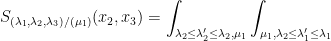
More generally, we can define the continuous skew Schur functions for of length , of length , and recursively by defining

and

for . Thus for instance

and

By expanding out the recursion, one obtains the analogue

of (6), and more generally one has

We will call the tuples in the first integral real Gelfand-Tsetlin patterns based at . The analogue of (8) is then

where the integral is over all real partitions of length , with Lebesgue measure.

By approximating various integrals by their Riemann sums, one can relate the continuous Schur functions to their discrete counterparts by the limiting formula

as for any length real partition and any , where

and

More generally, one has

as for any length real partition , any length real partition with , and any .

As a consequence of these limiting formulae, one expects all of the discrete identities above to have continuous counterparts. This is indeed the case; below the fold we shall prove the discrete and continuous identities in parallel. These are not new results by any means, but I was not able to locate a good place in the literature where they are explicitly written down, so I thought I would try to do so here (primarily for my own internal reference, but perhaps the calculations will be worthwhile to some others also).

Matrix identities as derivatives of determinant identities

The determinant of a square matrix obeys a large number of important identities, the most basic of which is the multiplicativity property

whenever are square matrices of the same dimension. This identity then generates many other important identities. For instance, if is an matrix and is an matrix, then by applying the previous identity to equate the determinants of and (where we will adopt the convention that denotes an identity matrix of whatever dimension is needed to make sense of the expressions being computed, and similarly for ) we obtain the Weinstein-Aronszajn determinant identity

This identity, which converts an determinant into an determinant, is very useful in random matrix theory (a point emphasised in particular by Deift), particularly in regimes in which is much smaller than .

Another identity generated from (1) arises when trying to compute the determinant of a block matrix

where is an matrix, is an matrix, is an matrix, and is an matrix. If is invertible, then we can manipulate this matrix via block Gaussian elimination as

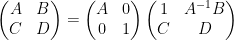
and on taking determinants using (1) we obtain the Schur determinant identity

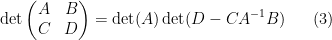
relating the determinant of a block-diagonal matrix with the determinant of the Schur complement of the upper left block . This identity can be viewed as the correct way to generalise the determinant formula

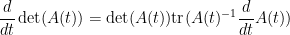
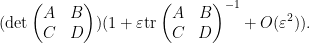
It is also possible to use determinant identities to deduce other matrix identities that do not involve the determinant, by the technique of matrix differentiation (or equivalently, matrix linearisation). The key observation is that near the identity, the determinant behaves like the trace, or more precisely one has

for any bounded square matrix and infinitesimal . (If one is uncomfortable with infinitesimals, one can interpret this sort of identity as an asymptotic as .) Combining this with (1) we see that for square matrices of the same dimension with invertible and invertible, one has

for infinitesimal . To put it another way, if is a square matrix that depends in a differentiable fashion on a real parameter , then we have the Jacobi formula

whenever is invertible. (Note that if one combines this identity with cofactor expansion, one recovers Cramer’s rule.)

Let us see some examples of this differentiation method. If we take the Weinstein-Aronszajn identity (2) and multiply one of the rectangular matrices by an infinitesimal , we obtain

applying (4) and extracting the linear term in (or equivalently, differentiating at and then setting ) we conclude the cyclic property of trace:

To manipulate derivatives and inverses, we begin with the Neumann series approximation

for bounded square and infinitesimal , which then leads to the more general approximation

for square matrices of the same dimension with bounded. To put it another way, we have

whenever depends in a differentiable manner on and is invertible.

We can then differentiate (or linearise) the Schur identity (3) in a number of ways. For instance, if we replace the lower block by for some test matrix , then by (4), the left-hand side of (3) becomes (assuming the invertibility of the block matrix)

while the right-hand side becomes

extracting the linear term in , we conclude that

As was an arbitrary matrix, we conclude from duality that the lower right block of is given by the inverse of the Schur complement:

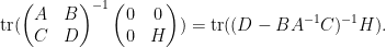
One can also compute the other components of this inverse in terms of the Schur complement by a similar method (although the formulae become more complicated). As a variant of this method, we can perturb the block matrix in (3) by an infinitesimal multiple of the identity matrix giving

By (4), the left-hand side is

From (5), we have

and so from (4) the right-hand side of (6) is

extracting the linear component in , we conclude the identity

which relates the trace of the inverse of a block matrix, with the trace of the inverse of one of its blocks. This particular identity turns out to be useful in random matrix theory; I hope to elaborate on this in a later post.

As a final example of this method, we can analyse low rank perturbations of a large () matrix , where is an matrix and is an matrix for some . (This type of situation is also common in random matrix theory, for instance it arose in this previous paper of mine on outliers to the circular law.) If is invertible, then from (1) and (2) one has the matrix determinant lemma

if one then perturbs by an infinitesimal matrix , we have

Extracting the linear component in as before, one soon arrives at

assuming that and are both invertible; as is arbitrary, we conclude (after using the cyclic property of trace) the Sherman-Morrison formula

for the inverse of a low rank perturbation of a matrix . While this identity can be easily verified by direct algebraic computation, it is somewhat difficult to discover this identity by such algebraic manipulation; thus we see that the “determinant first” approach to matrix identities can make it easier to find appropriate matrix identities (particularly those involving traces and/or inverses), even if the identities one is ultimately interested in do not involve determinants. (As differentiation typically makes an identity lengthier, but also more “linear” or “additive”, the determinant identity tends to be shorter (albeit more nonlinear and more multiplicative) than the differentiated identity, and can thus be slightly easier to derive.)

Exercise 1 Use the “determinant first” approach to derive the Woodbury matrix identity (also known as the binomial inverse theorem)

where is an matrix, is an matrix, is an matrix, and is an matrix, assuming that , and are all invertible.

Exercise 2 Let be invertible matrices. Establish the identity

and differentiate this in to deduce the identity

(assuming that all inverses exist) and thence

Rotating by then gives

which is useful for inverting a matrix that has been split into a self-adjoint component and a skew-adjoint component .

Random matrices: Universality of local spectral statistics of non-Hermitian matrices

Van Vu and I have just uploaded to the arXiv our paper “Random matrices: Universality of local spectral statistics of non-Hermitian matrices“. The main result of this paper is a “Four Moment Theorem” that establishes universality for local spectral statistics of non-Hermitian matrices with independent entries, under the additional hypotheses that the entries of the matrix decay exponentially, and match moments with either the real or complex gaussian ensemble to fourth order. This is the non-Hermitian analogue of a long string of recent results establishing universality of local statistics in the Hermitian case (as discussed for instance in this recent survey of Van and myself, and also in several other places).

The complex case is somewhat easier to describe. Given a (non-Hermitian) random matrix ensemble of matrices, one can arbitrarily enumerate the (geometric) eigenvalues as , and one can then define the -point correlation functions to be the symmetric functions such that

In the case when is drawn from the complex gaussian ensemble, so that all the entries are independent complex gaussians of mean zero and variance one, it is a classical result of Ginibre that the asymptotics of near some point as and is fixed are given by the determinantal rule

for and

for , where is the reproducing kernel

(There is also an asymptotic for the boundary case , but it is more complicated to state.) In particular, we see that for almost every , which is a manifestation of the well-known circular law for these matrices; but the circular law only captures the macroscopic structure of the spectrum, whereas the asymptotic (1) describes the microscopic structure.

Our first main result is that the asymptotic (1) for also holds (in the sense of vague convergence) when is a matrix whose entries are independent with mean zero, variance one, exponentially decaying tails, and which all match moments with the complex gaussian to fourth order. (Actually we prove a stronger result than this which is valid for all bounded and has more uniform bounds, but is a bit more technical to state.) An analogous result is also established for real gaussians (but now one has to separate the correlation function into components depending on how many eigenvalues are real and how many are strictly complex; also, the limiting distribution is more complicated, being described by Pfaffians rather than determinants). Among other things, this allows us to partially extend some known results on complex or real gaussian ensembles to more general ensembles. For instance, there is a central limit theorem of Rider which establishes a central limit theorem for the number of eigenvalues of a complex gaussian matrix in a mesoscopic disk; from our results, we can extend this central limit theorem to matrices that match the complex gaussian ensemble to fourth order, provided that the disk is small enough (for technical reasons, our error bounds are not strong enough to handle large disks). Similarly, extending some results of Edelman-Kostlan-Shub and of Forrester-Nagao, we can show that for a matrix matching the real gaussian ensemble to fourth order, the number of real eigenvalues is with probability for some absolute constant .

There are several steps involved in the proof. The first step is to apply the Girko Hermitisation trick to replace the problem of understanding the spectrum of a non-Hermitian matrix, with that of understanding the spectrum of various Hermitian matrices. The two identities that realise this trick are, firstly, Jensen’s formula

that relates the local distribution of eigenvalues to the log-determinants , and secondly the elementary identity

that relates the log-determinants of to the log-determinants of the Hermitian matrices

The main difficulty is then to obtain concentration and universality results for the Hermitian log-determinants . This turns out to be a task that is analogous to the task of obtaining concentration for Wigner matrices (as we did in this recent paper), as well as central limit theorems for log-determinants of Wigner matrices (as we did in this other recent paper). In both of these papers, the main idea was to use the Four Moment Theorem for Wigner matrices (which can now be proven relatively easily by a combination of the local semi-circular law and resolvent swapping methods), combined with (in the latter paper) a central limit theorem for the gaussian unitary ensemble (GUE). This latter task was achieved by using the convenient Trotter normal form to tridiagonalise a GUE matrix, which has the effect of revealing the determinant of that matrix as the solution to a certain linear stochastic difference equation, and one can analyse the distribution of that solution via such tools as the martingale central limit theorem.

The matrices are somewhat more complicated than Wigner matrices (for instance, the semi-circular law must be replaced by a distorted Marchenko-Pastur law), but the same general strategy works to obtain concentration and universality for their log-determinants. The main new difficulty that arises is that the analogue of the Trotter norm for gaussian random matrices is not tridiagonal, but rather Hessenberg (i.e. upper-triangular except for the lower diagonal). This ultimately has the effect of expressing the relevant determinant as the solution to a nonlinear stochastic difference equation, which is a bit trickier to solve for. Fortunately, it turns out that one only needs good lower bounds on the solution, as one can use the second moment method to upper bound the determinant and hence the log-determinant (following a classical computation of Turan). This simplifies the analysis on the equation somewhat.

While this result is the first local universality result in the category of random matrices with independent entries, there are still two limitations to the result which one would like to remove. The first is the moment matching hypotheses on the matrix. Very recently, one of the ingredients of our paper, namely the local circular law, was proved without moment matching hypotheses by Bourgade, Yau, and Yin (provided one stays away from the edge of the spectrum); however, as of this time of writing the other main ingredient – the universality of the log-determinant – still requires moment matching. (The standard tool for obtaining universality without moment matching hypotheses is the heat flow method (and more specifically, the local relaxation flow method), but the analogue of Dyson Brownian motion in the non-Hermitian setting appears to be somewhat intractible, being a coupled flow on both the eigenvalues and eigenvectors rather than just on the eigenvalues alone.)

Pythagoras’ theorem

My colleague Ricardo Pérez-Marco showed me a very cute proof of Pythagoras’ theorem, which I thought I would share here; it’s not particularly earth-shattering, but it is perhaps the most intuitive proof of the theorem that I have seen yet.

In the above diagram, a, b, c are the lengths BC, CA, and AB of the right-angled triangle ACB, while x and y are the areas of the right-angled triangles CDB and ADC respectively. Thus the whole triangle ACB has area x+y.

Now observe that the right-angled triangles CDB, ADC, and ACB are all similar (because of all the common angles), and thus their areas are proportional to the square of their respective hypotenuses. In other words, (x,y,x+y) is proportional to . Pythagoras’ theorem follows.