One of the oldest and most fundamental concepts in mathematics is the line. Depending on exactly what mathematical structures we want to study (algebraic, geometric, topological, order-theoretic, etc.), we model lines nowadays by a variety of standard mathematical objects, such as the real line  , the complex line
  , the projective line
  , the extended real line
 ![{}[-\infty,+\infty]](https://s0.wp.com/latex.php?latex=%7B%7D%5B-%5Cinfty%2C%2B%5Cinfty%5D&bg=ffffff&fg=545454&s=0&c=20201002) , the affine line
, the affine line  , the continuum
  , the long line
  , etc. We also have discrete versions of the line, such as the natural numbers
  , the integers
  , and the ordinal
  , as well as compact versions of the line, such as the unit interval
 ![{}[0,1]](https://s0.wp.com/latex.php?latex=%7B%7D%5B0%2C1%5D&bg=ffffff&fg=545454&s=0&c=20201002) or the unit circle
or the unit circle  . Finally we have discrete and compact versions of the line, such as the cyclic groups
  and the discrete intervals
  and
and  . By taking Cartesian products we then obtain higher-dimensional objects such as Euclidean space
  , the standard lattice
  , the standard torus
  , and so forth. These objects of course form the background on which a very large fraction of modern mathematics is set.
Broadly speaking, the line has three major families of structures on it:
- Geometric structures, such as a metric or a measure, completeness, scales (coarse and fine), rigid motions (translations and reflection), similarities (dilation, affine maps), and differential structures (tangent bundle, etc.);
- Algebraic structures, such group, ring, or field structures, and everything else that comes from those categories (e.g. subgroups, homomorphisms, involutions, etc.); and
- One-dimensional structures, such as order, a length space structure (in particular, path-connectedness structure), a singleton generator, the Archimedean property, the ability to use mathematical induction (i.e. well-ordering), convexity, or the ability to disconnect the line by removing a single point.
Of course, these structures are inter-related, and it is an important phenomenon that a mathematical concept which appears to be native to one structure, can often be equivalently defined in terms of other structures. For instance, the absolute value  of an integer
  can be defined geometrically as the distance from 0 to , algebraically as the index of the subgroup
  of the integers generated by n, or one-dimensionally as the number of integers between 0 and (including 0, but excluding ). This equivalence of definitions becomes important when one wants to work in more general contexts in which one or more of the above structures is missing or otherwise weakened.
What I want to talk about today is an important toy model for the line (in any of its incarnations), in which the geometric and algebraic structures are enhanced (and become neatly nested and recursive), at the expense of the one-dimensional structure (which is largely destroyed). This model has many different names, depending on what field of mathematics one is working in and which structures one is interested in. In harmonic analysis it is called the dyadic model, the Walsh model, or the Cantor group model; in number theory and arithmetic geometry it is known as the function field model; in topology it is the Cantor space model; in probability it is the martingale model; in metric geometry it is the ultrametric, tree, or non-Archimedean model; in algebraic geometry it is the Puiseux series model; in additive combinatorics it is the bounded torsion or finite field model; in computer science and information theory it is the Hamming cube model; in representation theory it is the Kashiwara crystal model. Let me arbitrarily select one of these terms, and refer to all of these models as dyadic models for the line (or of objects derived from the line). While there is often no direct link between a dyadic model and a non-dyadic model, dyadic models serve as incredibly useful laboratories in which to gain insight and intuition for the “real-world” non-dyadic model, since one has much more powerful and elegant algebraic and geometric structure to play with in this setting (though the loss of one-dimensional structure can be a significant concern). Perhaps the most striking example of this is the three-line proof of the Riemann hypothesis in the function field model of the integers, which I will discuss a little later.
— Dyadic integers and reals —
Very broadly speaking, one of the key advantages that dyadic models offer over non-dyadic models is that they do not have any “spillover” from one scale to the next. This spillover is introduced to us all the way back in primary school, when we learn about the algorithms for decimal notation arithmetic: long addition, long subtraction, long multiplication, and long division. In decimal notation, the notion of scale is given to us by powers of ten (with higher powers corresponding to coarse scales, and lower powers to fine scales), but in order to perform arithmetic properly in this notation, we must constantly “carry” digits from one scale to the next coarser scale, or conversely to “borrow” digits from one scale to the next finer one. These interactions between digits from adjacent scales (which in modern terminology, would be described as cocycles) make the arithmetic operations look rather complicated in decimal notation, although one can at least isolate the fine-scale behaviour from the coarse-scale digits (but not vice versa) through modular arithmetic. (To put it a bit more algebraically, the integers or real numbers can quotient out the coarse scales via normal subgroups (or ideals) such as  , but do not have a corresponding normal subgroup or ideal to quotient out the fine scales.)
It is thus natural to look for models of arithmetic in which this spillover is not present. One is first exposed to such models in high school, when the arithmetic of polynomials in one unknown  is introduced (i.e. one works with rings such as
 ![{\Bbb Z}[t]](https://s0.wp.com/latex.php?latex=%7B%5CBbb+Z%7D%5Bt%5D&bg=ffffff&fg=545454&s=0&c=20201002) or
or ![{\Bbb R}[t]](https://s0.wp.com/latex.php?latex=%7B%5CBbb+R%7D%5Bt%5D&bg=ffffff&fg=545454&s=0&c=20201002) rather than or ). For instance, to quotient one polynomial by another, one uses the polynomial long division (or synthetic division) algorithm, which is formally identical to long division for integers in decimal notation but without all the borrowing from one scale to the next. Here scales are represented by powers of , rather than powers of 10. As with the reals or integers, the coarse scales can be contained in a normal subgroups (and ideals) such as
rather than or ). For instance, to quotient one polynomial by another, one uses the polynomial long division (or synthetic division) algorithm, which is formally identical to long division for integers in decimal notation but without all the borrowing from one scale to the next. Here scales are represented by powers of , rather than powers of 10. As with the reals or integers, the coarse scales can be contained in a normal subgroups (and ideals) such as ![t^d \cdot {\Bbb R}[t]](https://s0.wp.com/latex.php?latex=t%5Ed+%5Ccdot+%7B%5CBbb+R%7D%5Bt%5D&bg=ffffff&fg=545454&s=0&c=20201002) , but now the fine scales can also be contained in normal subgroups (though not ideals) such as
, but now the fine scales can also be contained in normal subgroups (though not ideals) such as  , the group generated by
  (i.e. the group of polynomials of degree less than
  ). (From a category theory perspective, things are better here because various short exact sequences involving the scales are now split.)
Now, polynomial rings such as or are a bit “too big” to serve as models for or (unless one adjoins some infinitesimals, but that’s another story), as they have one more dimension. One can get a more accurate model by considering the decimal representation again, which identifies natural numbers as polynomials over the space of digits  . This space is not closed under addition (which is what causes spillover in the first place); but we can remedy this by replacing this space of digits with the cyclic group
  . This gives us the model
 ![({\Bbb Z}/10{\Bbb Z})[t]](https://s0.wp.com/latex.php?latex=%28%7B%5CBbb+Z%7D%2F10%7B%5CBbb+Z%7D%29%5Bt%5D&bg=ffffff&fg=545454&s=0&c=20201002) for the integers; this is the decimal representation without the operation of carrying. If we follow the usual decimal notation and identify polynomials in with strings of digits in the usual manner (e.g. identifying
for the integers; this is the decimal representation without the operation of carrying. If we follow the usual decimal notation and identify polynomials in with strings of digits in the usual manner (e.g. identifying  with 32) then we obtain a number system which is similar, but not quite identical, to the integers. For instance, 66 + 77 now equals 33 rather than 143; 25*4 now equals 80 rather than 100; and so forth. Note that unlike the natural numbers, the space of polynomials is already closed under negation and so there is no need to introduce negative numbers; for instance, in this system we have -12 = 98. I’ll refer to as the “base 10 dyadic” model for the integers (somewhat annoyingly, the term “10-adic” is already taken to mean something slightly different).
There is also a base 10 dyadic model for the real numbers, in which we allow infinitely many negative powers of t but only finitely many positive powers in t; in other words, the model is  , the ring of formal Laurent series in
  . This ring again differs slightly from the reals; for instance,
  is now no longer equal to
  (in fact, they differ by
  ). So the decimal notation maps onto the positive real axis
  , but there is a small amount of non-injectivity caused by this map.
The base 10 dyadic models for the reals and integers are not particularly accurate, due to the presence of zero divisors in the underlying base ring . For instance, we have  in this model. One can do a lot better by working over a finite field F, such as the field
  of two elements. This gives us dyadic models
 ![F[t]](https://s0.wp.com/latex.php?latex=F%5Bt%5D&bg=ffffff&fg=545454&s=0&c=20201002) and
and  for the integers and reals respectively which turn out to be much closer analogues than the base 10 model. For instance, , like the integers, is an Euclidean domain, and is a field. (In the binary case
  , the addition operation is just bitwise XOR, and multiplication is bitwise convolution.) We can also model many other non-dyadic objects, as the following table illustrates:
| Non-dyadic |
Dyadic |
| Integers |
Polynomials |
Rationals  |
Rational functions  |
| Reals |
Laurent polynomials |
Unit circle  |
![F((1/t))/F[t] \equiv \frac{1}{t} F[\frac{1}{t}]](https://s0.wp.com/latex.php?latex=F%28%281%2Ft%29%29%2FF%5Bt%5D+%5Cequiv+%5Cfrac%7B1%7D%7Bt%7D+F%5B%5Cfrac%7B1%7D%7Bt%7D%5D&bg=ffffff&fg=545454&s=0&c=20201002) |
 |
![t^d \cdot F[t]](https://s0.wp.com/latex.php?latex=t%5Ed+%5Ccdot+F%5Bt%5D&bg=ffffff&fg=545454&s=0&c=20201002) |
Cyclic group  |
Vector space  |
Finite field  |
Finite field ![F[t]/p(t) \cdot F[t]](https://s0.wp.com/latex.php?latex=F%5Bt%5D%2Fp%28t%29+%5Ccdot+F%5Bt%5D&bg=ffffff&fg=545454&s=0&c=20201002) |
| Absolute value |
(Exponential of) degree |
| Plane wave |
Walsh function
|
| Wavelet |
Haar wavelet |
| Gaussian |
Step function |
| Ball |
Dyadic interval |
| Heat operators |
Martingale conditional expectations |
| Band-limited |
Locally constant |
| Interval / arithmetic progression |
Subspace / subgroup |
| Bohr set |
Hyperplane |
Recall that we can define the absolute value (or norm) of an integer n as the index of the subgroup  of the integers. Exactly the same definition can be applied to the dyadic model of the integers; the absolute value of an element
 ![n \in F[t]](https://s0.wp.com/latex.php?latex=n+%5Cin+F%5Bt%5D&bg=ffffff&fg=545454&s=0&c=20201002) can then be seen to equal
can then be seen to equal  , where
  is the degree of t in n (with the convention that 0 has a degree of
  and thus an absolute value of 0). For instance, in the binary case,
  (or 1011) has a norm of 8. Like the absolute value on the integers, the absolute value on the dyadic model of the integers is multiplicative and obeys the triangle inequality, giving rise to a metric on by the usual formula
  . In fact, we have something better than a metric, namely an ultrametric; in the dyadic world, the triangle inequality

can be strengthened to the ultratriangle inequality
 .
.
One can then uniquely extend this absolute value multiplicatively to the dyadic model of the reals, which is given by the same formula  , where is now understood to be the highest exponent of t which appears in the expansion of n (or of no such exponent appears). Thus for instance in the binary case
  (or
(or  ) has a norm of 1/2. Just as with the real line, this absolute value turns the dyadic real line into a complete metric space. The metric space then generates balls
  , which in the binary case are identifiable with dyadic intervals. The fact that we have an ultrametric instead of a metric means that the balls enjoy a very useful nesting property, which is unavailable in the non-dyadic setting: if two balls intersect, then the larger one must necessarily contain the smaller one.
On the other hand, all the “one-dimensional” structure of the real line is lost when one passes to the dyadic model. For instance, the dyadic real line is still locally compact, but not locally connected; the topology is instead locally that of a Cantor space. There is no natural notion of order on the dyadic integers or real line, and the metric is non-Archimedean. Related to this, mathematical induction no longer applies to the dyadic integers. Nevertheless, and somewhat counter-intuitively, one can go remarkably far in mimicking many features of the integers and real numbers without using any one-dimensional structure. I’ll try to illustrate this in a number of contexts.
— Dyadic models in harmonic analysis —
Let us first compare the harmonic analysis of the dyadic and non-dyadic models. Lebesgue measure dx is the unique Haar measure on the real line which assigns a measure of 1 to the unit interval ![[0,1]](https://s0.wp.com/latex.php?latex=%5B0%2C1%5D&bg=ffffff&fg=545454&s=0&c=20201002) . Similarly, the dyadic real line , there is a unique Haar measure dx which assigns a measure of 1 to the unit ball B(0,1). Indeed, this measure can be defined by pulling back Lebesgue measure on the positive real axis via the decimal map which maps elements of to the corresponding base |F| expansion in the reals (e.g. in the binary case,
. Similarly, the dyadic real line , there is a unique Haar measure dx which assigns a measure of 1 to the unit ball B(0,1). Indeed, this measure can be defined by pulling back Lebesgue measure on the positive real axis via the decimal map which maps elements of to the corresponding base |F| expansion in the reals (e.g. in the binary case,  would be mapped to
  ).
).
The general theory of harmonic analysis on locally compact abelian groups then shows that there is a theory of the Fourier transform on the dyadic real line , which turns out to be closely analogous to that on the non-dyadic real line . (There is also a Fourier theory relating the dyadic integers with the dyadic unit circle ![F((1/t))/F[t] \equiv \frac{1}{t} \cdot F[\frac{1}{t}]](https://s0.wp.com/latex.php?latex=F%28%281%2Ft%29%29%2FF%5Bt%5D+%5Cequiv+%5Cfrac%7B1%7D%7Bt%7D+%5Ccdot+F%5B%5Cfrac%7B1%7D%7Bt%7D%5D&bg=ffffff&fg=545454&s=0&c=20201002) , which we leave to the reader.) Recall that the Fourier transform on the real line is built out of the 1-periodic character
, which we leave to the reader.) Recall that the Fourier transform on the real line is built out of the 1-periodic character  defined by
  by the formula

for all well-behaved  (e.g. absolutely integrable f). Similarly, the Fourier transform on (assuming F to be a prime field
  for simplicity) can be built out of the 1-periodic character
  defined by

(which would be a square wave in the binary case) using almost exactly the same formula, namely

for all well-behaved  . One can then show that this dyadic Fourier transform (known as the Walsh-Fourier transform in the binary case) enjoys all the usual algebraic properties that the non-dyadic Fourier transform does – for instance, it reacts with convolution, translation, modulation, and dilation in exactly the same way as its non-dyadic counterpart, and also enjoys a perfect analogue of Plancherel’s theorem. (It also has a more pleasant fast Fourier transform algorithm than its non-dyadic counterpart, as one no longer needs the additional step of taking care of the spillover from one scale to the next.) In fact, the dyadic structure makes the harmonic analysis on somewhat simpler than that on , because of the ability to have perfect phase space localisation. In the real line, it is well-known that a function and its Fourier transform cannot simultaneously be compactly supported without vanishing completely (because if a function was compactly supported, then its Fourier transform would be a real analytic function, which cannot be compactly supported without vanishing completely, due to analytic continuation). However, analytic continuation is a highly “one-dimensional” property (it exploits connectedness). Furthermore, it is not a robust property, and it is possible to have functions f on the real line such that f and its Fourier transform are “almost compactly supported”, or more precisely rapidly decreasing; the Gaussian function
  , which is its own Fourier transform, is a particularly good example. In the dyadic world, the analogue of the Gaussian function is the step function
  , which is also its own Fourier transform, and thus demonstrates that it is possible for a function and its Fourier transform to both be compactly supported. More generally, it is possible for a function to be supported on a dyadic interval I, and for its Fourier transform to be supported on another dyadic interval J, as long as the uncertainty principle
  is respected. One can use these “Walsh wave packets” (which include the Haar wavelets and Radamacher functions as special cases) to elegantly and efficiently perform time-frequency analysis in the dyadic setting. This has proven to be an invaluable model to work with before tackling the more interesting time-frequency problems in the non-dyadic setting (such as those relating to Carleson’s theorem, or to various multilinear singular integrals), as many technical headaches (such as those involving “Schwartz tails”) are absent in the dyadic setting, while the time-frequency combinatorics (which is really the heart of the matter) stays largely intact. (To give just one example, the Shannon sampling theorem collapses in the dyadic setting to the trivial statement that a function which is locally constant on dyadic intervals of length
  , can be reconstructed exactly by sampling that function at intervals of .) See these lecture notes of Pereyra or of myself for more discussion. In some cases one can in fact deduce a non-dyadic harmonic analysis result directly from a dyadic one via some sort of averaging argument (or the 1/3 translation trick of Michael Christ, which is the observation that every non-dyadic interval (in, say, [0,1]) is contained either in a dyadic interval of comparable size, or the 1/3 translation of a dyadic interval of comparable size). In particular the “Bellman function” approach to harmonic analysis often proceeds via this averaging, as the Bellman function method requires a recursive dyadic structure (or a continuous heat kernel-type structure) in order to work properly. In general, though, the dyadic argument only serves as a model “road map” for the non-dyadic argument, rather than a formal component. There are only a few cases known where a dyadic result in harmonic analysis has not shown the way towards proving the non-dyadic analogue; one of these exceptions is the problem of establishing a nonlinear analogue of Carleson’s theorem, which was achieved in the dyadic setting but remains open in the non-dyadic setting.
— Dyadic models in PDE —
Let us now leave harmonic analysis and turn to dyadic and non-dyadic models of other parts of mathematics. I should briefly discuss PDEs, which is one field in which the dyadic models have proven to have only a limited impact (though the Katz-Pavlovic dyadic model for the Euler and Navier-Stokes equations is perhaps a counterexample). This is partly because, in contrast to harmonic analysis, the analysis of PDEs does heavily exploit the one-dimensionality of the real line (and in particular, the time axis), for instance via the use of continuity arguments or monotonicity formulae. Nevertheless one can still obtain some partial analogues of various PDE objects, most notably those connected to the heat equation, as long as one is willing to work with dyadic notions of time. For instance, in the binary case , the dyadic analogue of the heat operator  when
when  is a power of 4 would be the conditional expectation operator to the
  -algebra generated by dyadic intervals of length
  . These conditional expectations are nested in n, yielding a martingale structure. There is in fact a very strong (and well known) analogy between heat operators and conditional expectations with respect to a martingale; to give just one example, the sharp Young’s inequality on the real line can be proven by a heat flow method (ensuring that a certain multilinear expression is monotone along heat flow), and the corresponding sharp Young’s inequality on or
  can similarly be proven (with a somewhat shorter proof) by a nested conditional expectation argument.
— Dyadic models in additive combinatorics —
We now briefly turn to additive combinatorics. Here, it is often convenient for combinatorial reasons to work not on an infinite additive group such as or , but in a finite additive group. In the non-dyadic setting, one usually uses a cyclic group such as  ; in the dyadic setting, one uses a vector space such as (one should think of F as being fixed, e.g. or
  , and n as being large). A general philosophy is that as long as these two groups have roughly the same size (i.e.
  ), then the additive combinatorics of these two groups will be broadly analogous, even if algebraically the groups are rather different (the former can be generated by a single generator, but most elements have large order, whereas the latter needs many generators, and all elements have small order). But the dyadic model tends to be significantly more tractable for a number of reasons. Most obviously, the group is also a vector space, and thus one can apply the powerful tools of linear algebra. A cyclic group only has some partial (and messy) analogues of linear algebraic tools; for instance, in cyclic groups generalised arithmetic progressions are somewhat analogous to vector spaces spanned by a given set of vectors, has a lot of subgroups; dually, Bohr sets (level sets of one or more characters) play a role in cyclic groups analogous to the intersection of one or more hyperplanes in . See this survey paper of Green for further discussion. Another useful feature of the group is the presence of flags of subspaces, e.g. the coordinate flag

which allows one in some cases to prove combinatorial facts in by an induction on dimension, and to use tools related to such flags such as the combinatorial technique of compression. See this previous blog post for some examples of this.
Very recently, though, Ben Green and I have discovered that the lack of one-dimensionality in the finite field model can make that model less tractable than the cyclic group model in certain technical senses. For instance, Gowers’ celebrated proof of Szemerèdi’s theorem does not quite work in finite field models because of this little wrinkle. This seems to have something to do with the (still poorly understood) analogy between nilsequences in the non-dyadic setting, and polynomials in the dyadic setting. Hopefully we’ll have more to say about this in the future.
— Dyadic models in algebraic combinatorics —
I’ll now touch briefly on the role of dyadic models in algebraic combinatorics. Here it seems that many algebraic questions that are over the field or collapse to purely combinatorial questions once one “tropicalises” by passing to a dyadic model field, such as the field of Puiseux series  . Furthermore (and rather miraculously), certain questions have identical answers in the dyadic and non-dyadic settings, thus allowing one to use combinatorial gadgets to solve algebraic problems. For instance, the question of understanding the possible relationships between eigenvalues of a sum A+B of Hermitian matrices, with the eigenvalues of A and B separately, is a non-trivial algebraic problem; but by passing to the dyadic model of Puiseux series and extracting the leading exponents (which does not affect the final answer) it was shown by Speyer that the problem collapses to the combinatorial problem of locating a honeycomb between the three sets of putative eigenvalues. (This fact, as well as the one below, had been established earlier by Knutson and myself by a much more indirect method.) There is also a discrete (representation-theoretic) counterpart to this phenomenon; the question of computing tensor product multiplicities for the unitary group U(n) is also a non-trivial algebraic problem, in large part due to the “mixing” between basis elements of irreducible representations when one takes tensor products and then decomposes again into irreducibles (in the case n=2, this mixing is described by the Clebsch-Gordan coefficients; the situation is more complicated in higher n due to multiplicities in the decomposition). But if one replaces the notion of a representation with the “dyadic” model of a crystal representation, the mixing is eliminated (without affecting the multiplicities), and it was shown by Henriques and Kamnitzer that the problem of computing tensor product multiplicities again collapses to a honeycomb problem. It would be interesting to get a more general explanation of why these phenomena occur.
— Dyadic models in number theory —
Finally, I want to discuss the role of dyadic models in number theory – a topic which has in fact been the subject of at least one entire graduate text. In contrast to the other settings discussed above, there is a fantastic disparity in number theory between our understanding of the dyadic model and that of the non-dyadic model; several of the most famous problems in non-dyadic number theory (e.g. Riemann hypothesis, Fermat’s last theorem, twin prime conjecture, abc conjecture, factorisation of large numbers) are surprisingly easy to solve in the dyadic world (see e.g. Zhang’s talk for the dyadic version of FLT), but nobody knows how to convert the dyadic arguments to the non-dyadic setting (although the converse step of converting non-dyadic arguments to dyadic ones is usually rather straightforward). One notable exception here is the parity problem, which has resisted progress in both dyadic and non-dyadic settings.
Let’s now turn to the Riemann hypothesis. Classically, number theory has focused on the multiplicative structure of the ring of integers . After factoring out the group of units  , we usually restrict attention to the positive integers
  . In the dyadic model, we study the multiplicative structure of the ring of polynomials for some finite field F. After factoring out the group
  of units, we can restrict attention to the monic polynomials
 ![F[t]_m](https://s0.wp.com/latex.php?latex=F%5Bt%5D_m&bg=ffffff&fg=545454&s=0&c=20201002) . As the ring of polynomials is a Euclidean domain, it has unique factorisation, and in particular every monic polynomial can be expressed uniquely (up to permutation) as the product of irreducible monic polynomials, which we shall call prime polynomials.We can analyse the problem of counting primes in by using zeta functions, in complete analogy with the integer case. The Riemann zeta function is of course given by
. As the ring of polynomials is a Euclidean domain, it has unique factorisation, and in particular every monic polynomial can be expressed uniquely (up to permutation) as the product of irreducible monic polynomials, which we shall call prime polynomials.We can analyse the problem of counting primes in by using zeta functions, in complete analogy with the integer case. The Riemann zeta function is of course given by

(for  ) and we introduce the analogous zeta function
![\zeta_{F[t]}(s) := \sum_{n \in F[t]_m} \frac{1}{|n|^s}](https://s0.wp.com/latex.php?latex=%5Czeta_%7BF%5Bt%5D%7D%28s%29+%3A%3D+%5Csum_%7Bn+%5Cin+F%5Bt%5D_m%7D+%5Cfrac%7B1%7D%7B%7Cn%7C%5Es%7D&bg=ffffff&fg=545454&s=0&c=20201002) .
.
In the integers, unique factorisation gives the identity
where  is the von Mangoldt function, defined to equal
  when d is the power of a prime p and 0 otherwise. Taking the Mellin transform of this identity, we conclude that
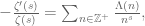
which is the fundamental identity linking the zeroes of the zeta function to the distribution of the primes. We can do the same thing in the dyadic case, obtaining the identity
![-\frac{\zeta'_{F[t]}(s)}{\zeta_{F[t]}(s)} = \sum_{n \in F[t]_m} \frac{\Lambda_{F[t]}(n)}{|n|^s},](https://s0.wp.com/latex.php?latex=-%5Cfrac%7B%5Czeta%27_%7BF%5Bt%5D%7D%28s%29%7D%7B%5Czeta_%7BF%5Bt%5D%7D%28s%29%7D+%3D+%5Csum_%7Bn+%5Cin+F%5Bt%5D_m%7D+%5Cfrac%7B%5CLambda_%7BF%5Bt%5D%7D%28n%29%7D%7B%7Cn%7C%5Es%7D%2C&bg=ffffff&fg=545454&s=0&c=20201002) (1)
(1)
where the von Mangoldt function ![\Lambda_{F[t]}(n)](https://s0.wp.com/latex.php?latex=%5CLambda_%7BF%5Bt%5D%7D%28n%29&bg=ffffff&fg=545454&s=0&c=20201002) for F[t] is defined as
for F[t] is defined as  when n is the power of a prime polynomial p, and 0 otherwise.
So far, the dyadic and non-dyadic situations are very closely analogous. But now we can do something special in the dyadic world: we can compute the zeta function explicitly by summing by degree. Indeed, we have
![\zeta_{F[t]}(s) = \sum_{d=0}^\infty \sum_{n \in F[t]_m: \hbox{deg}(n)=d} \frac{1}{|F|^{ds}}](https://s0.wp.com/latex.php?latex=%5Czeta_%7BF%5Bt%5D%7D%28s%29+%3D+%5Csum_%7Bd%3D0%7D%5E%5Cinfty+%5Csum_%7Bn+%5Cin+F%5Bt%5D_m%3A+%5Chbox%7Bdeg%7D%28n%29%3Dd%7D+%5Cfrac%7B1%7D%7B%7CF%7C%5E%7Bds%7D%7D&bg=ffffff&fg=545454&s=0&c=20201002) .
.
The number of monic polynomials of degree d is  . Summing the geometric series, we obtain an exact formula for the zeta function:
![\zeta_{F[t]}(s) = (1 - |F|^{s-1})^{-1}](https://s0.wp.com/latex.php?latex=%5Czeta_%7BF%5Bt%5D%7D%28s%29+%3D+%281+-+%7CF%7C%5E%7Bs-1%7D%29%5E%7B-1%7D&bg=ffffff&fg=545454&s=0&c=20201002) .
.
In particular, the Riemann hypothesis for F[t] is a triviality – there are clearly no zeroes whatsoever! Inserting this back into (1) and comparing coefficients, one soon ends up with an exact prime number theorem for F[t]:
![\sum_{n \in F[t]_m: \hbox{deg}(n)=d} \Lambda(n) = |F|^d \log |F|](https://s0.wp.com/latex.php?latex=%5Csum_%7Bn+%5Cin+F%5Bt%5D_m%3A+%5Chbox%7Bdeg%7D%28n%29%3Dd%7D+%5CLambda%28n%29+%3D+%7CF%7C%5Ed+%5Clog+%7CF%7C&bg=ffffff&fg=545454&s=0&c=20201002)
which quickly implies that the number of prime polynomials of degree d is  . (One can generalise the above analysis to other varieties over finite fields, leading ultimately to the (now-proven) Weil conjectures, which include the “Riemann hypothesis for function fields”.)
Another example of a problem which is hard in non-dyadic number theory but trivial in dyadic number theory is factorisation. In the integers, it is not known whether a number which is n digits long can be factored (probabilistically) in time polynomial in n (the best known algorithm for large n, the number field sieve, takes a little longer than  time); indeed, the presumed hardness of factoring underlies many popular cryptographic protocols such as RSA. However, in with F fixed, a polynomial f of degree n can be factored (probabilistically) in time polynomial in n by the following three-stage algorithm:
- Compute the gcd of f and its derivative f’ using the Euclidean algorithm (which is polynomial time in the degree). This locates all the repeated factors of f, and lets one quickly reduce to the case when f is squarefree. (This trick is unavailable in the integer case, due to the lack of a good notion of derivative.)
- Observe (from Cauchy’s theorem) that for any prime polynomial g of degree d, we have
 . Thus the polynomial
  contains the product of all the primes of this degree (and of all primes of degree dividing d); indeed, by the exact prime number theorem and a degree count, these are the only possible factors of . It is easy to compute the remainder of modulo f in polynomial time, and then one can compute gcd of f with in polynomial time also. This essentially isolates the prime factors of a fixed degree, and quickly lets one reduce to the case when f is the product of distinct primes of the same degree d. (Here we have exploited the fact that there are many primes with exactly the same norm – which is of course highly false in the integers. Similarly in Step 3 below.)
- Now we apply the Cantor-Zassenhaus algorithm. Let us assume that |F| is odd (the case |F|=2 can be treated by a modification of this method). By computing
 for randomly selected g, we can generate some random square roots a of 1 modulo f (thanks to Cauchy’s theorem and the Chinese remainder theorem; there is also a small chance we generate a non-invertible element, but this is easily dealt with). These square roots a will be either +1 or -1 modulo each of the prime factors of f. If we take the gcd of f with a+1 or a-1 we have a high probability of splitting up the prime factors of f; doing this a few times one soon isolates all the prime factors separately.
— Conclusion —
As the above whirlwind tour hopefully demonstrates, dyadic models for the integers, reals, and other “linear” objects show up in many different areas of mathematics. In some areas they are an oversimplified and overly easy toy model; in other areas they get at the heart of the matter by providing a model in which all irrelevant technicalities are stripped away; and in yet other areas they are a crucial component in the analysis of the non-dyadic case. In all of these cases, though, it seems that the contribution that dyadic models provide in helping us understand the non-dyadic world is immense.


37 comments
Comments feed for this article
27 July, 2007 at 8:27 am
John Armstrong
Would it then be fair to say that the difference between dyadic models and non-dyadic models is parallel to the difference between abelian and non-abelian gauge field theories?
You seem to indicate that one can use a dyadic analogue to get at the heart of a problem, and then try to adapt that proof to the original setting. In that approach, one must get a handle on the messiness that comes with using a nontrivial cocycle that crosses the scales. To what extent can an appropriate classification of “bundles” (or “gerbes”) help this effort?
27 July, 2007 at 9:23 am
Terence Tao
Dear John,
That’s an interesting analogy. Dyadic models are suppressing cocycles rather than commutators, but there is certainly a similar theme in that both types of objects destroy “perfect decoupling” in some sense. But the cocycles tend to be a little more pleasant to deal with, because they seem to be a bit more unidirectional or “nilpotent”. For instance, one can add a small number to a large number to move the large number to the next largest scale, but you can’t get the large number to modify the small number in a similar manner. Whereas in a non-abelian gauge theory, if the gauge group is simple then you’re going to see every component of the gauge group interact, eventually, with every other. This “nilpotency” seems to be an important enabler for letting one generalise a dyadic argument to a non-dyadic argument; often the key is to attend to the scales in the right order (either working on coarse scales first and only then tackling the fine, or vice versa, or doing a preliminary sparsification of the scales to make the non-dyadic model look more dyadic), and to make sure that the various errors caused by spillover effects don’t blow up while doing so.
Regarding classification of bundles and gerbes, I feel that the concepts of dyadic vs non-dyadic are still rather vague and certainly not at the point where one can use cohomological tools to concretely identify what obstruction the non-dyadic world has that the dyadic world doesn’t. Part of the problem is that we don’t really have a family of continuous deformations from the dyadic world to the non-dyadic world (except possibly in the algebraic combinatorics setting, where various quantum algebras, as well as the process of tropicalisation and detropicalisation, seem to be filling this role). This, by the way, would be a fantastic way to prove the Riemann hypothesis for integers, by continuously deforming from the function field model! This seems wildly optimistic to me, though.
27 July, 2007 at 9:33 am
Dyadic models and magnetic order « Entertaining Research
[…] models and magnetic order Terry Tao gives a whirlwind tour of dyadic models: … an important toy model for the line (in any of its incarnations), in which the geometric […]
27 July, 2007 at 10:04 am
John Armstrong
But isn’t a commutator a sort of cocycle? Maybe a more apt analogy is conformal field theory, where one must add central charges (a cocycle) to properly lift the representation theories at hand.
27 July, 2007 at 2:42 pm
Terence Tao
Hmm, I never thought of them that way before, but I guess you’re right, a commutator is indeed a special type of cocycle. On the other hand, it seems to a somewhat different type of cocycle from that which appears in the interactions between scales for the integers and reals (which don’t appear to have any particularly non-commutative structure in them :-).
My knowledge of CFTs is pretty minimal, but the central charge c appears to be a deformation parameter for some sort of algebra, which does look (on a superficial level, at least) like how the quantum parameter q is a deformation parameter for the universal enveloping algebra for, say, sl_n, which is how the Kashiwara crystal representations arise as deformations of the representation theory of a Lie group. So the analogy might have some substance to it, at least for the dyadic models that come up in algebraic combinatorics. [On the other hand, from a physical perspective q is usually interpreted as a “temperature” rather than a “charge”, which fits with the more general philosophy of interpreting these scale-mixing cocycles as being some sort of messy, entropy-producing phenomenon.]
27 July, 2007 at 3:59 pm
Top Posts « WordPress.com
[…] Dyadic models One of the oldest and most fundamental concepts in mathematics is the line. Depending on exactly what mathematical […] […]
30 July, 2007 at 8:56 am
Doug
Hi Terence,
Your use of “tropicalises” suggests to me either tropical geometry or tropical algebra.
Are these also referred to as Min-Plus Algebra [Geometry], related to Max-Plus algebra? I am more familiar with the latter.
The terminology is similar but not identical:
dioid algebra rather than dyadic
and
idempotent semiring rather than nilpotent.
These algebras are extensions of mathematical game theory.
I am most familiar with:
1 – ‘Dynamic Noncooperative Game Theory’, Tamer Basar, Geert Jan Olsder
2 – Max-Plus at Work: …”, Bernd Heidergott, Geert Jan Olsder, and Jacob van der Woude
3 – Some of the arxiv papers of Stephane Gaubert, INRIA.
I suspect some type of rigorous relation [beyond my ability], since John von Neumann had ‘rings of operators’ algebra for physics and ‘minimax’ game theory for engineering and economics?
They may also be related via trajectory curves [ballistics] through Euler?
30 July, 2007 at 8:43 pm
Terence Tao
Dear Doug,
There is indeed a connection. If you take the semi-ring of polynomials![{\Bbb R}_+[t]](https://s0.wp.com/latex.php?latex=%7B%5CBbb+R%7D_%2B%5Bt%5D&bg=ffffff&fg=545454&s=0&c=20201002) with non-negative coefficients in one variable t (which can be thought of as one of the dyadic models of the line), then the degree map
with non-negative coefficients in one variable t (which can be thought of as one of the dyadic models of the line), then the degree map  is a homomorphism from that semi-ring to the max-plus algebra of the natural numbers:
  ,
,  . If you want the max-plus algebra of the reals rather than the natural numbers, use Puiseux series instead of polynomials. The paper of Speyer referenced above exploits this connection.
3 August, 2007 at 10:54 pm
Doug
Hi Terence,
I remain stunned at the simple elegance of your equations using a degree map.
I had thought that the more complicated mathematics of dynamic noncoopertive game theory would be needed.
You seem to have unified the Nobel categories of Physics and Economics?
Thanks for the Speyer reference.
4 August, 2007 at 7:59 am
Terence Tao
Dear Doug,
Mathematics is the common language of all the sciences, so it is actually not that surprising that a single mathematical concept can appear two unrelated disciplines. As an analogy, a Harry Potter novel and a legal contract may share some words of English in common (including perhaps some rare or unusual words), but this is not exactly a “unification” of the two documents. In particular, reading one is unlikely to inform the other, except possibly for the fact that you may need to look up the same word in the dictionary in both cases.
On the other hand, if two documents had several sentences in common (up to trivial rewordings), then there is a more serious connection. Similarly, if two areas of science are using the same (or very similar) theorems about mathematical objects, then it can become profitable to consider the analogies between those two areas.
23 September, 2007 at 11:36 am
Phil Isett
Dear Terence,
I did a little work on a certain generalization of Haar Wavelets to (compact) groups which were “solvable” in a sense like that of Galois Theory; formal Laurent series over a finite field being just one example. I just gave a seminar on it at the University of Maryland, where I’m currently a senior. (The seminar didn’t go too well for various reasons, including both a concurrent football game and my own inexperience in this sort of thing)
After reading this entry I thought you might have been interested in the work. If you’d care, I could send you the paper in a PDF file.
~Phil Isett
11 December, 2007 at 5:23 pm
The Walsh model for M_2^* Carleson « What’s new
[…] of ours on the return times theorem of Bourgain, in which the Fourier transform is replaced by its dyadic analogue, the Walsh-Fourier transform. This model estimate is established by the now-standard techniques of […]
17 December, 2007 at 5:34 pm
Multi-linear multipliers associated to simplexes of arbitrary length « What’s new
[…] using a trace formula (a nonlinear analogue to Plancherel’s formula). Also, the “dyadic” or “function field” model of the conjecture is known, by a modification of […]
24 March, 2008 at 10:31 am
Dvir’s proof of the finite field Kakeya conjecture « What’s new
[…] 1999, Wolff proposed a simpler finite field analogue of the Kakeya conjecture as a model problem that avoided all the technical issues involving […]
27 July, 2008 at 2:24 pm
Tate’s proof of the functional equation « What’s new
[…] analogues in the p-adic completions of the rationals . (This is analogous to my discussion of dyadic models, although the p-adics are still characteristic 0 and are not as dyadic as their function field […]
8 May, 2010 at 1:47 pm
254B, Lecture Notes 4: Equidistribution of polynomials over finite fields « What’s new
[…] when ) and also in number theory; but they also serve as an important simplified “dyadic model” for the integers. See this survey article of Green for further discussion of this […]
25 June, 2010 at 6:44 pm
The uncertainty principle « What’s new
[…] fraction of the time”; for a precise definition, see my book with Van Vu). However, there are dyadic models of Euclidean domains, such as the field of formal Laurent series in a variable over a finite […]
19 October, 2010 at 9:18 pm
bilboy
Most of the number systems have a basis of the form , essentially the basis is a geometric series.
Can there be a bijection between integers and an additive basis, i.e, can every integer be represented as , where $b_i$ is not an geometric series (does not grow as fast as b^n for some fixed b). Can we restrict $b_i$ to be an arithmetic series with varying gap. If not for the entire integer set, does such a bijection for a fraction of integers?
20 October, 2010 at 8:52 pm
LifeIsChill
There is a motivic description of some of the algebraic structures starting with the line you are commenting on. Does your description have any connection to motivic models?
9 March, 2011 at 1:31 pm
Rohlin’s problem on strongly mixing systems « What’s new
[…] is a “dyadic” (or more precisely, “triadic”) model for the integers (cf. this earlier blog post of mine). In other words: Theorem 2 There exists a -system that is strongly -mixing but not strongly […]
22 October, 2011 at 9:30 pm
binary transforms | Peter's ruminations
[…] See https://terrytao.wordpress.com/2007/07/27/dyadic-models/ […]
20 May, 2012 at 11:25 pm
Heuristic limitations of the circle method « What’s new
[…] located. On the other hand, the situation is significantly more promising if one works in the function field model in which the integers are replaced by the ring of polynomials of one variable over a finite field, […]
23 June, 2012 at 8:47 am
dyadic models in number theory–would NSA *want* to suppress results? | Peter's ruminations
[…] https://terrytao.wordpress.com/2007/07/27/dyadic-models/ […]
26 October, 2014 at 6:18 pm
Mark Keith’s constrained writing | The Daily Pochemuchka
[…] easily appreciated as very very hard because we can immediately think of toy examples (to bastardize Tao), for instance writing a ten-word sentence that reads the same forwards and backwards instead of a […]
15 December, 2014 at 12:23 pm
Abdelmalek Abdesselam
That’s a terrific post!! It’s too bad however that the discussion did not include sections on the dyadic models in probability and in physics. In physics, a ubiquitous framework for trying to understand a wide variety of phenomena is the quantum field theory formalism and at the heart of it is Wilson’s renormalization group. There too there are Euclidean (non-dyadic) models and their hierarchical (dyadic) version. Wilson himself referred to dyadic models as “the approximate recursion”. Working with this toy model was in fact crucial to the discoveries made by Wilson (such as the epsilon-expansion). I explained some of this in
http://arxiv.org/abs/1311.4897 In probability theory the dyadic models such as the branching Brownian motion or random walk are a useful toy model for the so-called Gaussian free field. A similar idea is that of Mandelbrot cascades.
27 December, 2014 at 8:50 pm
What are examples of good toy models in mathematics? | CL-UAT
[…] comment on another question reminded me of this old post of Terence Tao’s about toy models. I really like the idea of using toy models of a difficult object to understand it […]
15 July, 2015 at 2:44 pm
Cycles of a random permutation, and irreducible factors of a random polynomial | What's new
[…] the analogy between integers and polynomials over a finite field , discussed for instance in this previous post; this is the simplest case of the more general function field analogy between number fields and […]
18 March, 2017 at 12:04 pm
curiousquery.
You say in Cantor-Zassenhaus algorithm. Let us assume that |F| is odd (the case |F|=2 can be treated by a modification of this method). By computing $g^{(|F|^d-1)/2} \hbox{ mod } f$ for randomly selected g, we can generate some random square roots a of 1 modulo f and gcd of a +/- 1 mod f factors f with high probability. Will this work over Z? then we would have a probabilistic reduction from factoring to quadratic residue which is an open problem.
22 March, 2017 at 5:56 am
Terence Tao
As mentioned in the blog post, this step relies crucially on the fact that all the prime factors of a given degree have exactly the same magnitude (so the same exponent
  works regardless of what the factors are). In the integer case, the prime factors have different magnitudes, and it is not clear how to proceed this way. (If we somehow were able to compute the Euler totient function
  of the number
  we wished to factor, we would be in much better shape, but this may well be as hard as the original factoring problem.)
3 January, 2018 at 2:20 pm
The Dyadic Riemann hypothesis - Quantum Calculus
[…] The Dyadic group of integers is not so familiar to us that the circle. It is a much simpler space however as it is quantized, (we have a smallest translation, a dynamical system which is also called the “adding machine”), it is still a compact space and a natural limit of one-dimensional geometric spaces in the Barycentric limit. Also, its dual, the Prüfer group does not have any interesting primes. The Prüfer group is the spectrum of the Koopman operator of the adding machine. I got to this when looking at renormalizations of random Jacobi matrices. The Dyadic group appeared there naturally as a limit of a 2:1 integral extension in ergodic theory: the group translation is called the von Neumann-Kakutani system. The limiting operators are almost periodic operators defined over that system. The spectra are on located Julia sets, the density of states are the equilibrium measures on that sets. In some sense, these Jacobi operators define “quantized Julia sets” as they are operators for which the spectra are Julia sets. Some other mathematical connections to the dyadic world are discussed here, in a blog of Tao from more than 10 years ago. […]
17 June, 2019 at 2:51 pm
L
Are there models derived from non-one dimensional objects such as the plane?
5 November, 2020 at 9:23 pm
.
Is there a dyadic and non-dyadic interpretation for matrix products?
1 December, 2020 at 7:51 am
Dyadic models in number theory and "spillover" ~ MathOverflow ~ mathubs.com
[…] a classic blog post, Tao discusses the appearance of "dyadic models" in various guises in various areas of […]
31 December, 2020 at 2:37 am
Onsprctrsl
Would the laplacian operator in spectral graph theory and geometry be considered non-dyadic? If so what would be the dyadic version? Any references?
31 December, 2020 at 12:20 pm
Terence Tao
The spectrum of most Laplacians are not concentrated in a lacunary set such as the powers of two, so would not be considered dyadic operators, although it is often profitable to treat them as if they were dyadic using the device of Littlewood-Paley theory. Given a dyadic mesh structure on a space one can create a dyadic analogue of a Laplacian (or more generally fractional powers of the Laplacian), though they do not have as much of a geometric interpretation as the more traditional Laplacians. See for instance https://arxiv.org/abs/2004.10940 for a recent treatment of such operators.
5 March, 2023 at 4:03 pm
Chasing integers
Why are polynomials ‘the’ dyadic model for integers? Are there other ‘types’ of models for integers other than dyadic models?
9 March, 2023 at 6:42 am
Terence Tao
It comes down to the fact that there are only two types of global fields: number fields and function fields. The integers are the ring of integers for the simplest number field , while polynomials
 ![{\bf F}_q[T]](https://s0.wp.com/latex.php?latex=%7B%5Cbf+F%7D_q%5BT%5D&bg=ffffff&fg=545454&s=0&c=20201002) over a finite field are the ring of integers for the simplest function field
over a finite field are the ring of integers for the simplest function field  . (One can axiomatically define what a global field is in terms of valuations without reference to either number fields or function fields.)