Classically, the fundamental object of study in algebraic geometry is the solution set


to multiple algebraic equations

in multiple unknowns  in a field
  , where the
  are polynomials of various degrees
  . We adopt the classical perspective of viewing
  as a set (and specifically, as an algebraic set), rather than as a scheme. Without loss of generality we may order the degrees in non-increasing order:

We can distinguish between the underdetermined case  , when there are more unknowns than equations; the determined case
  when there are exactly as many unknowns as equations; and the overdetermined case
  , when there are more equations than unknowns.
Experience has shown that the theory of such equations is significantly simpler if one assumes that the underlying field is algebraically closed , and so we shall make this assumption throughout the rest of this post. In particular, this covers the important case when  is the field of complex numbers (but it does not cover the case
  of real numbers – see below).
From the general “soft” theory of algebraic geometry, we know that the algebraic set is a union of finitely many algebraic varieties, each of dimension at least  , with none of these components contained in any other. In particular, in the underdetermined case
  , there are no zero-dimensional components of , and thus is either empty or infinite.
Now we turn to the determined case  , where we expect the solution set to be zero-dimensional and thus finite. Here, the basic control on the solution set is given by Bezout’s theorem. In our notation, this theorem states the following:
Theorem 1 (Bezout’s theorem) Let  . If is finite, then it has cardinality at most
  .
.
This result can be found in any introductory algebraic geometry textbook; it can for instance be proven using the classical tool of resultants. The solution set will be finite when the two polynomials  are coprime, but can (and will) be infinite if share a non-trivial common factor.
By defining the right notion of multiplicity on (and adopting a suitably “scheme-theoretic” viewpoint), and working in projective space rather than affine space, one can make the inequality  an equality. However, for many applications (and in particular, for the applications to combinatorial incidence geometry), the upper bound usually suffices.
Bezout’s theorem can be generalised in a number of ways. For instance, the restriction on the finiteness of the solution set can be dropped by restricting attention to  , the union of the zero-dimensional irreducible components of :
Corollary 2 (Bezout’s theorem, again) Let . Then has cardinality at most .
Proof: We factor  into irreducible factors (using unique factorisation of polynomials). By removing repeated factors, we may assume are square-free. We then write
  ,
,  where
where  is the greatest common divisor of and
  are coprime. Observe that the zero-dimensional component of
  is contained in
  , which is finite from the coprimality of . The claim follows.
It is also not difficult to use Bezout’s theorem to handle the overdetermined case  in the plane:
Corollary 3 (Bezout’s theorem, yet again) Let  . Then has cardinality at most .
Proof: We may assume all the  are square-free. We write
  , where
  is coprime to
  and
and  divides (and also
  ). We then write
  , where
  is coprime to
  and
and  divides (and also ). Continuing in this fashion we obtain a factorisation
  . One then observes that is contained in the set
  , which by Theorem 1 has cardinality at most
  . Since
  and
and  , the claim follows.
Remark 1 Of course, in the overdetermined case one generically expects the solution set to be empty, but if there is enough degeneracy or numerical coincidence then non-zero solution sets can occur. In particular, by considering the case when  and
and  we see that the bound can be sharp in some cases. However, one can do a little better in this situation; by decomposing
  into irreducible components, for instance, one can improve the upper bound of slightly to
  . However, this improvement seems harder to obtain in higher dimensions (see below).
Bezout’s theorem also extends to higher dimensions. Indeed, we have
Theorem 4 (Higher-dimensional Bezout’s theorem) Let  . If is finite, then it has cardinality at most
  .
.
This is a standard fact, and can for instance be proved from the more general and powerful machinery of intersection theory. A typical application of this theorem is to show that, given a degree  polynomial
  over the reals, the number of connected components of
  is
is  . The main idea of the proof is to locate a critical point
  inside each connected component, and use Bezout’s theorem to count the number of zeroes of the polynomial map
  . (This doesn’t quite work directly because some components may be unbounded, and because the fibre of
  at the origin may contain positive-dimensional components, but one can use truncation and generic perturbation to deal with these issues; see my recent paper with Solymosi for further discussion.)
Bezout’s theorem can be extended to the overdetermined case as before:
Theorem 5 (Bezout’s inequality) Let  . Then has cardinality at most .
Remark 2 Theorem 5 ostensibly only controls the zero-dimensional components of , but by throwing in a few generic affine-linear forms to the set of polynomials  (thus intersecting with a bunch of generic hyperplanes) we can also control the total degree of all the
  -dimensional components of for any fixed . (Again, by using intersection theory one can get a slightly more precise bound than this, but the proof of that bound is more complicated than the arguments given here.)
This time, though, it is a slightly non-trivial matter to deduce Theorem 5 from Theorem 4, due to the standard difficulty that the intersection of irreducible varieties need not be irreducible (which can be viewed in some ways as the source of many other related difficulties, such as the fact that not every algebraic variety is a complete intersection), and so one cannot evade all irreducibility issues merely by assuming that the original polynomials are irreducible. Theorem 5 first appeared explicitly in the work of Heintz.
As before, the most systematic way to establish Theorem 5 is via intersection theory. In this post, though, I would like to give a slightly more elementary argument (essentially due to Schmid), based on generically perturbing the polynomials in the problem ; this method is less powerful than the intersection-theoretic methods, which can be used for a wider range of algebraic geometry problems, but suffices for the narrow objective of proving Theorem 5. The argument requires some of the “soft” or “qualitative” theory of algebraic geometry (in particular, one needs to understand the semicontinuity properties of preimages of dominant maps), as well as basic linear algebra. As such, the proof is not completely elementary, but it uses only a small amount of algebraic machinery, and as such I found it easier to understand than the intersection theory arguments.
Theorem 5 is a statement about arbitrary polynomials . However, it turns out (in the determined case , at least) that upper bounds on  are Zariski closed properties, and so it will suffice to establish this claim for generic polynomials . On the other hand, it is possible to use duality to deduce such upper bounds on from a Zariski open condition, namely that a certain collection of polynomials are linearly independent. As such, to verify the generic case of this open condition, it suffices to establish this condition for a single family of polynomials, such as a family of monomials, in which case the condition can be verified by direct inspection. Thus we see an example of the somewhat strange strategy of establishing the general case from a specific one, using the generic case as an intermediate step.
Remark 3 There is an important caveat to note here, which is that these theorems only hold for algebraically closed fields, and in particular can fail over the reals  . For instance, in
  , the polynomials


have degrees  respectively, but their common zero locus
  has cardinality
  . In some cases one can safely obtain incidence bounds in by embedding inside
  , but as the above example shows, one needs to be careful when doing so.
— 1. The determined case —
We begin by establishing Theorem 4. Fix  . If one wishes, one can dispose of the trivial case
  and assume
  , although this is not strictly necessary for the argument below.
As mentioned in the introduction, the first idea is to generically perturb the  . To this end, let
  be the vector space
  , where
  is the vector space of all polynomials
  of degree at most
  ; thus is the configuration space of all possible . This is a finite-dimensional vector space over with an explicit dimension
  which we will not need to compute here. The set
  in (1) can thus be viewed as the fibre over
  of the algebraic set
  , defined as


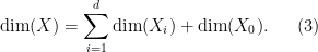
This algebraic set is cut out by  polynomial equations on
  and thus is the union of finitely many algebraic varieties
  , each of which has codimension at most in . In particular,
  .
.
Consider one of the components  of
of  . Its projection
  in will be Zariski dense in its closure
  , which is necessarily an irreducible variety since is, and the projection map from to will, by definition, be a dominant map. By basic algebraic geometry, the preimages in of a point in will generically have dimension
  (i.e. this dimension will occur outside of a algebraic subset of of positive codimension), and even in the non-generic case will have dimension at least . Since , we thus see that the only components that can contribute to the zero-dimensional set are those with
  . Now, the projection map is a dominant map between two varieties of the same dimension, and is thus generically finite, with the preimages generically having some constant cardinality
  , and non-generically the preimages have a zero-dimensional component of at most . (Topologically, one can see this claim (at least in the model case ) as follows. Any isolated point
  in a non-generic preimage must perturb to a zero-dimensional set or to an empty set in nearby preimages, since is closed. On a generic preimage, must perturb to a zero-dimensional set (for if it generically perturbs to the empty set, the dimension of will be too small); since a generic preimage has points, we conclude that the non-generic preimage can contain at most isolated points. For a more detailed proof of this claim, see Proposition 1 of Heintz’s paper.)
As a consequence of this analysis, we see that the generic fibre always has at least as many zero-dimensional components as a non-generic fibre, and so to establish Theorem 4, it suffices to do so for generic .
Now take to be generic. We know that generically, the set is finite; we seek to bound its cardinality  by
by  . To do this, we dualise the problem. Let
  be the space of all affine-linear forms
  ; this is a
  -dimensional vector space. We consider the set
  of all affine-linear forms
  whose kernel
  intersects . This is a union of hyperplanes in , and is thus a hypersurface of degree . Thus, to upper bound the size of , it suffices to upper bound the degree of the hypersurface , and this can be done by finding a non-zero polynomial of controlled degree that vanishes identically on . The point of this observation is that the property of a polynomial being non-zero is a Zariski-open condition, and so we have a chance of establishing the generic case from a special case.
Now let us look for a (generically non-trivial) polynomial of degree at most  that vanishes on . The idea is to try to dualise the assertion that the monomials
  with
with  for all
  generically span the function ring of , to become a statement about .
Let be a sufficiently large integer (any integer larger than  will do, actually), and let
  be the space of all polynomials
  of degree at most . This is a finite-dimensional vector space over , generated by the monomials with
  non-negative integers adding up to at most . We can split as a direct sum

where for  ,
,  is generated by those monomials of degree at most
  with for all
  and with
  , and
, and  is generated by those monomials with for all . In particular,
Also observe that

Now let  be an affine-linear form, and consider the sum
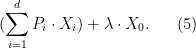
This is a subspace of for large enough. In view of (2), we see that this sum can equal all of in the case when  and
and  . From (3), the property of (5) spanning all of is a Zariski-open condition, and thus we see that (5) spans for generic choices of and .
On the other hand, suppose that  , thus
  for some
  . Then observe that each factor of (5) lies in the hyperplane
  of , and so (5) does not span in this case. Thus, for generic , we see that (5) spans for generic but not for any in .
The property of (5) spanning is equivalent to a certain resultant-like determinant of a  matrix being non-zero, where the rows are given by the generators of
  and
and  . For generic , this determinant is a non-trivial polynomial in which vanishes on ; an inspection of the matrix reveals that this determinant has degree
  in . Thus we have found a non-trivial polynomial of degree that vanishes on , and the claim follows.
— 2. The overdetermined case —
Now we establish Theorem 5. Fix , and let  be the union of all the positive-dimensional components of , thus
  .
.
The main idea here is to perturb to be a regular sequence of polynomials outside of . More precisely, we have
Lemma 6 (Regular sequence) For any  , one can find polynomials
  , such that for each
  ,
,  is a linear combination of
  (and thus has degree at most ), with the coefficient being non-zero, and the set
  in
in  has dimension at most
  (in the sense that it is covered by finitely many varieties of dimension at most ).
Proof: We establish this claim by induction on  . For
. For  the claim follows by setting
  . Now suppose inductively that
  , and that
  have already been found with the stated properties for
  .
.
By construction, the polynomials are linear combinations of  . Thus, on the set
  , the polynomials
  can only simultaneously vanish on the zero-dimensional set
  . On the other hand, each irreducible component of has dimension
  , which is positive. Thus it is not possible for to simultaneously vanish on any of these components. If one then sets
  to be a generic linear combination of , then we thus see that will also not vanish on any of these components, and so has dimension at most . Also, generically the
  coefficient of is non-zero, and the claim follows.
From the above lemma (with  ) we see that
  is contained in the set
  . By Theorem 4, the latter set has cardinality at most , and the claim follows.


20 comments
Comments feed for this article
23 March, 2011 at 11:03 pm
Allen Knutson
the intersection of irreducible varieties need not be irreducible (which is closely related to the fact that not every algebraic variety is a complete intersection)
I’m having trouble guessing what you’re thinking of here. Complete intersections are already often reducible.
24 March, 2011 at 4:56 am
David Speyer
I think what Terry is thinking is the following: Here is a flawed proof that every variety is a complete intersection. For concreteness, I will “prove” that every curve in 3-space is a complete intersection. For large enough degree, there is a polynomial
  vanishing on
  such that
  is irreducible. Let
  be a point of
  not on
  . For large enough degree, there is a polynomial
  vanishing on
  and not at
  , and we can take
  irreducible. So
  is a proper subvariety of
  , containing
  . If the intersection of irreducible varieties was always irreducible, it would have to be
  .
.
I’ve seen several students find this proof. There is usually a lot more detail in the parts where you check that and
and  can be found with the required properties, which makes the error less conspicuous.
[Yes, this is the type of thing I had in mind; in the counterfactual world where intersections of irreducibles were irreducible, many other things in algebraic geometry would oversimplify, in particular all varieties would be complete intersections. I’ve reworded the text a little bit. – T.]
24 March, 2011 at 6:21 am
Miguel Lacruz
It seems that there is a compiling error right after 2. The overdetermined case. Now we establish Theorem […]
[Fixed, thanks – T.]
6 April, 2011 at 9:20 pm
Fay
Hi,
Can I say that the infinite union of isolated point is not algebraic? That seems true but I can’t prove it .While in the affine A^1 , and A^2 space , this is true . But I don’t know if it still holds for higher dimension? Thanks !
Fay
15 April, 2011 at 11:47 pm
Evgeniy
Hi,
Every algebraic variety has a degree, which is a strictly positive integer (and it is finite). This degree is just a coefficient with dominant term of Hilbert-Samuel polynomial. For 0-dimensional cycle C the degree coincides with number of points (counting the multiplicity). You can see the last affirmation, for example, coincidering the interpolation at the points of C. So infinite union of points can not be algebraic.
16 April, 2011 at 1:55 am
Fay
What do you mean by “last affirmation”?
16 April, 2011 at 8:17 pm
Evgeniy
I am sorry, english is not my native language. I mean this: “For 0-dimensional cycle C the degree coincides with number of points (counting the multiplicity).”
16 April, 2011 at 10:27 pm
Fay
Thanks ! I am guessing you may assume that the infinite union of isolated points must be a 0 dimensional cycle , therefore a contradiction with a finite degree ,right? But i am confused that why it must be 0 dimensional ? Thanks!
14 April, 2011 at 5:37 pm
Erik
Is there a special form of Bezout’s theorem for ‘sparse’ polynomials?
For example, suppose that for each
  , and
, and  with
with  large, while each
  contains products like
  ,
,  , and
, and  .
.
15 April, 2011 at 8:30 am
Terence Tao
I don’t believe there are substantial gains to the Bezout bound from sparsity alone; for instance, in the plane, Bezout’s inequality is basically an equality (if one counts intersection points with multiplicity, assuming no common factors between polynomials, and working in an algebraically closed field of course).
This isn’t quite the same thing, but there is a variant of the Bezout bound known as the combinatorial nullstellensatz that prevents the zero set of a polynomial from containing a large Cartesian product if a certain coefficient of that polynomial is non-zero. This does give some sort of link between the combinatorial structure of algebraic sets and their sparsity, though the connection is not really of Bezout type.
15 April, 2011 at 11:44 am
Erik
Thanks Terrence.
Just after I wrote this I came accross a review
article that describes a very simple example, similar to the one I gave above (called a deficient system).
In the example, the polynomials contain all terms of the form
  ,
,  and
and  where the constants,
  , etc. are arbitrary. The Bezout bound is
  but the number of isolated solutions is
  .
.
I’d have to read a bit more on this, but it seems, as you suggest, that as things get more complicated the large gain over the Bezout bound may be lost very quickly.
Thanks again for your response and for this excellent blog.
The example is described on p. 212 of :
T. Y. Li,
Numerical solution of polynomial systems by homotopy continuation,
Handbook of Numerical Analysis, Volume 11, 2003, Pages 209-304.
Here’s the link,
http://www.sciencedirect.com/science/book/9780444512475
1 July, 2016 at 10:38 pm
Alperen ergur
Hi,
I am not sure if I understand the comment right but isn’t the mixed volume bounds of Bersntein’s theorem a big gain over Bezout?
It depends the Newton polytope which is some what sparsity.
15 July, 2011 at 7:32 pm
Pappus’s theorem and elliptic curves « What’s new
[…] One of the fundamental theorems about algebraic plane curves is Bézout’s theorem, which asserts that if a degree curve and a degree curve have no common component, then they intersect in at most points (and if the underlying field is algebraically closed, one works projectively, and one counts intersections with multiplicity, they intersect in exactly points). Thus, for instance, two distinct lines intersect in at most one point; a line and a conic section intersect in at most two points; two distinct conic sections intersect in at most four points; a line and an elliptic curve intersect in at most three points; two distinct elliptic curves intersect in at most nine points; and so forth. Bézout’s theorem is discussed in this previous post. […]
16 July, 2011 at 12:25 pm
Srivatsan Narayanan
In Theorem 5, shouldn’t the condition be the other way round?
[Corrected, thanks – T.]
18 July, 2011 at 5:40 am
Srivatsan Narayanan
Sorry to bother you much, but it seems that the post doesn’t reflect the correction :-)
[Oops; should be visible now. -T.]
25 September, 2012 at 1:17 pm
A partial converse to Bezout’s theorem « What’s new
[…] has many strengthenings, generalisations, and variants; see for instance this previous blog post on Bézout’s inequality. Bézout’s theorem asserts a fundamental algebraic dichotomy, of importance in […]
14 August, 2016 at 12:13 am
Anonymous
I wonder what can be said about the real case.
Is there a version of Theorem 5 that says that for some function f,
either V < f(D,k), where D is the max degree of the m polynomials,
or V_0 is infinite? Is there a polynomial bound for f?
14 August, 2016 at 2:01 am
Alperen ergur
I guess you would like to see Descartes Rule of Signs or Fewnomial Theory
14 August, 2016 at 2:21 am
gipi
Is there an equivalent of Bézout theorem for systems of trigonometric polynomials?
14 August, 2016 at 2:22 am
Anonymous
Hi Alperen, Could you be more specific?
Do you know any bound on f(D,k)?
As Terry mentioned, one cannot get the same bound as in the complex case, but I just wonder if one can get something in that neighborhood.