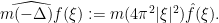
Perhaps the most fundamental differential operator on Euclidean space {{\bf R}^d} is the Laplacian

\displaystyle  \Delta := \sum_{j=1}^d \frac{\partial^2}{\partial x_j^2}.

The Laplacian is a linear translation-invariant operator, and as such is necessarily diagonalised by the Fourier transform

\displaystyle  \hat f(\xi) := \int_{{\bf R}^d} f(x) e^{-2\pi i x \cdot \xi}\ dx.

Indeed, we have

\displaystyle  \widehat{\Delta f}(\xi) = - 4 \pi^2 |\xi|^2 \hat f(\xi)

for any suitably nice function {f} (e.g. in the Schwartz class; alternatively, one can work in very rough classes, such as the space of tempered distributions, provided of course that one is willing to interpret all operators in a distributional or weak sense).

Because of this explicit diagonalisation, it is a straightforward manner to define spectral multipliers {m(-\Delta)} of the Laplacian for any (measurable, polynomial growth) function {m: [0,+\infty) \rightarrow {\bf C}}, by the formula

\displaystyle  \widehat{m(-\Delta) f}(\xi) := m( 4\pi^2 |\xi|^2 ) \hat f(\xi).

(The presence of the minus sign in front of the Laplacian has some minor technical advantages, as it makes {-\Delta} positive semi-definite. One can also define spectral multipliers more abstractly from general functional calculus, after establishing that the Laplacian is essentially self-adjoint.) Many of these multipliers are of importance in PDE and analysis, such as the fractional derivative operators {(-\Delta)^{s/2}}, the heat propagators {e^{t\Delta}}, the (free) Schrödinger propagators {e^{it\Delta}}, the wave propagators {e^{\pm i t \sqrt{-\Delta}}} (or {\cos(t \sqrt{-\Delta})} and {\frac{\sin(t\sqrt{-\Delta})}{\sqrt{-\Delta}}}, depending on one’s conventions), the spectral projections {1_I(\sqrt{-\Delta})}, the Bochner-Riesz summation operators {(1 + \frac{\Delta}{4\pi^2 R^2})_+^\delta}, or the resolvents {R(z) := (-\Delta-z)^{-1}}.

Each of these families of multipliers are related to the others, by means of various integral transforms (and also, in some cases, by analytic continuation). For instance:

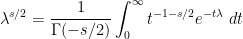
  1. Using the Laplace transform, one can express (sufficiently smooth) multipliers in terms of heat operators. For instance, using the identity

    \displaystyle  \lambda^{s/2} = \frac{1}{\Gamma(-s/2)} \int_0^\infty t^{-1-s/2} e^{-t\lambda}\ dt

    (using analytic continuation if necessary to make the right-hand side well-defined), with {\Gamma} being the Gamma function, we can write the fractional derivative operators in terms of heat kernels:

    \displaystyle  (-\Delta)^{s/2} = \frac{1}{\Gamma(-s/2)} \int_0^\infty t^{-1-s/2} e^{t\Delta}\ dt. \ \ \ \ \ (1)

  2. Using analytic continuation, one can connect heat operators {e^{t\Delta}} to Schrödinger operators {e^{it\Delta}}, a process also known as Wick rotation. Analytic continuation is a notoriously unstable process, and so it is difficult to use analytic continuation to obtain any quantitative estimates on (say) Schrödinger operators from their heat counterparts; however, this procedure can be useful for propagating identities from one family to another. For instance, one can derive the fundamental solution for the Schrödinger equation from the fundamental solution for the heat equation by this method.
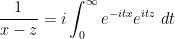
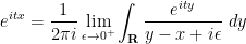
  3. Using the Fourier inversion formula, one can write general multipliers as integral combinations of Schrödinger or wave propagators; for instance, if {z} lies in the upper half plane {{\bf H} := \{ z \in {\bf C}: \hbox{Im} z > 0 \}}, one has

    \displaystyle  \frac{1}{x-z} = i\int_0^\infty e^{-itx} e^{itz}\ dt

    for any real number {x}, and thus we can write resolvents in terms of Schrödinger propagators:

    \displaystyle  R(z) = i\int_0^\infty e^{it\Delta} e^{itz}\ dt. \ \ \ \ \ (2)

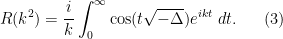
    In a similar vein, if {k \in {\bf H}}, then

    \displaystyle  \frac{1}{x^2-k^2} = \frac{i}{k} \int_0^\infty \cos(tx) e^{ikt}\ dt

    for any {x>0}, so one can also write resolvents in terms of wave propagators:

    \displaystyle  R(k^2) = \frac{i}{k} \int_0^\infty \cos(t\sqrt{-\Delta}) e^{ikt}\ dt. \ \ \ \ \ (3)

  4. Using the Cauchy integral formula, one can express (sufficiently holomorphic) multipliers in terms of resolvents (or limits of resolvents). For instance, if {t > 0}, then from the Cauchy integral formula (and Jordan’s lemma) one has

    \displaystyle  e^{itx} = \frac{1}{2\pi i} \lim_{\epsilon \rightarrow 0^+} \int_{\bf R} \frac{e^{ity}}{y-x+i\epsilon}\ dy

    for any {x \in {\bf R}}, and so one can (formally, at least) write Schrödinger propagators in terms of resolvents:

    \displaystyle  e^{-it\Delta} = - \frac{1}{2\pi i} \lim_{\epsilon \rightarrow 0^+} \int_{\bf R} e^{ity} R(y+i\epsilon)\ dy. \ \ \ \ \ (4)

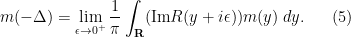
  5. The imaginary part of {\frac{1}{\pi} \frac{1}{x-(y+i\epsilon)}} is the Poisson kernel {\frac{\epsilon}{\pi} \frac{1}{(y-x)^2+\epsilon^2}}, which is an approximation to the identity. As a consequence, for any reasonable function {m(x)}, one has (formally, at least)

    \displaystyle  m(x) = \lim_{\epsilon \rightarrow 0^+} \frac{1}{\pi} \int_{\bf R} (\hbox{Im} \frac{1}{x-(y+i\epsilon)}) m(y)\ dy

    which leads (again formally) to the ability to express arbitrary multipliers in terms of imaginary (or skew-adjoint) parts of resolvents:

    \displaystyle  m(-\Delta) = \lim_{\epsilon \rightarrow 0^+} \frac{1}{\pi} \int_{\bf R} (\hbox{Im} R(y+i\epsilon)) m(y)\ dy. \ \ \ \ \ (5)

    Among other things, this type of formula (with {-\Delta} replaced by a more general self-adjoint operator) is used in the resolvent-based approach to the spectral theorem (by using the limiting imaginary part of resolvents to build spectral measure). Note that one can also express {\hbox{Im} R(y+i\epsilon)} as {\frac{1}{2i} (R(y+i\epsilon) - R(y-i\epsilon))}.

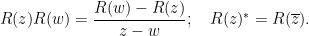
Remark 1 The ability of heat operators, Schrödinger propagators, wave propagators, or resolvents to generate other spectral multipliers can be viewed as a sort of manifestation of the Stone-Weierstrass theorem (though with the caveat that the spectrum of the Laplacian is non-compact and so the Stone-Weierstrass theorem does not directly apply). Indeed, observe the *-algebra type properties

\displaystyle  e^{s\Delta} e^{t\Delta} = e^{(s+t)\Delta}; \quad (e^{s\Delta})^* = e^{s\Delta}

\displaystyle  e^{is\Delta} e^{it\Delta} = e^{i(s+t)\Delta}; \quad (e^{is\Delta})^* = e^{-is\Delta}

\displaystyle  e^{is\sqrt{-\Delta}} e^{it\sqrt{-\Delta}} = e^{i(s+t)\sqrt{-\Delta}}; \quad (e^{is\sqrt{-\Delta}})^* = e^{-is\sqrt{-\Delta}}

\displaystyle  R(z) R(w) = \frac{R(w)-R(z)}{z-w}; \quad R(z)^* = R(\overline{z}).

Because of these relationships, it is possible (in principle, at least), to leverage one’s understanding one family of spectral multipliers to gain control on another family of multipliers. For instance, the fact that the heat operators {e^{t\Delta}} have non-negative kernel (a fact which can be seen from the maximum principle, or from the Brownian motion interpretation of the heat kernels) implies (by (1)) that the fractional integral operators {(-\Delta)^{-s/2}} for {s>0} also have non-negative kernel. Or, the fact that the wave equation enjoys finite speed of propagation (and hence that the wave propagators {\cos(t\sqrt{-\Delta})} have distributional convolution kernel localised to the ball of radius {|t|} centred at the origin), can be used (by (3)) to show that the resolvents {R(k^2)} have a convolution kernel that is essentially localised to the ball of radius {O( 1 / |\hbox{Im}(k)| )} around the origin.

In this post, I would like to continue this theme by using the resolvents {R(z) = (-\Delta-z)^{-1}} to control other spectral multipliers. These resolvents are well-defined whenever {z} lies outside of the spectrum {[0,+\infty)} of the operator {-\Delta}. In the model three-dimensional case {d=3}, they can be defined explicitly by the formula

\displaystyle  R(k^2) f(x) = \int_{{\bf R}^3} \frac{e^{ik|x-y|}}{4\pi |x-y|} f(y)\ dy

whenever {k} lives in the upper half-plane {\{ k \in {\bf C}: \hbox{Im}(k) > 0 \}}, ensuring the absolute convergence of the integral for test functions {f}. (In general dimension, explicit formulas are still available, but involve Bessel functions. But asymptotically at least, and ignoring higher order terms, one simply replaces {\frac{e^{ik|x-y|}}{4\pi |x-y|}} by {\frac{e^{ik|x-y|}}{c_d |x-y|^{d-2}}} for some explicit constant {c_d}.) It is an instructive exercise to verify that this resolvent indeed inverts the operator {-\Delta-k^2}, either by using Fourier analysis or by Green’s theorem.

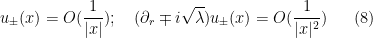
Henceforth we restrict attention to three dimensions {d=3} for simplicity. One consequence of the above explicit formula is that for positive real {\lambda > 0}, the resolvents {R(\lambda+i\epsilon)} and {R(\lambda-i\epsilon)} tend to different limits as {\epsilon \rightarrow 0}, reflecting the jump discontinuity in the resolvent function at the spectrum; as one can guess from formulae such as (4) or (5), such limits are of interest for understanding many other spectral multipliers. Indeed, for any test function {f}, we see that

\displaystyle  \lim_{\epsilon \rightarrow 0^+} R(\lambda+i\epsilon) f(x) = \int_{{\bf R}^3} \frac{e^{i\sqrt{\lambda}|x-y|}}{4\pi |x-y|} f(y)\ dy

and

\displaystyle  \lim_{\epsilon \rightarrow 0^+} R(\lambda-i\epsilon) f(x) = \int_{{\bf R}^3} \frac{e^{-i\sqrt{\lambda}|x-y|}}{4\pi |x-y|} f(y)\ dy.

Both of these functions

\displaystyle  u_\pm(x) := \int_{{\bf R}^3} \frac{e^{\pm i\sqrt{\lambda}|x-y|}}{4\pi |x-y|} f(y)\ dy

solve the Helmholtz equation

\displaystyle  (-\Delta-\lambda) u_\pm = f, \ \ \ \ \ (6)

but have different asymptotics at infinity. Indeed, if
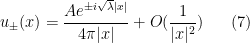
 {\int_{{\bf R}^3} f(y)\ dy = A}, then we have the asymptotic

\displaystyle  u_\pm(x) = \frac{A e^{\pm i \sqrt{\lambda}|x|}}{4\pi|x|} + O( \frac{1}{|x|^2}) \ \ \ \ \ (7)

as {|x| \rightarrow \infty}, leading also to the Sommerfeld radiation condition

\displaystyle  u_\pm(x) = O(\frac{1}{|x|}); \quad (\partial_r \mp i\sqrt{\lambda}) u_\pm(x) = O( \frac{1}{|x|^2}) \ \ \ \ \ (8)

where {\partial_r := \frac{x}{|x|} \cdot \nabla_x} is the outgoing radial derivative. Indeed, one can show using an integration by parts argument that {u_\pm} is the unique solution of the Helmholtz equation (6) obeying (8) (see below). {u_+} is known as the outward radiating solution of the Helmholtz equation (6), and {u_-} is known as the inward radiating solution. Indeed, if one views the function {u_\pm(t,x) := e^{-i\lambda t} u_\pm(x)} as a solution to the inhomogeneous Schrödinger equation

\displaystyle  (i\partial_t + \Delta) u_\pm = - e^{-i\lambda t} f

and using the de Broglie law that a solution to such an equation with wave number {k \in {\bf R}^3} (i.e. resembling {A e^{i k \cdot x}} for some amplitide {A}) should propagate at (group) velocity {2k}, we see (heuristically, at least) that the outward radiating solution will indeed propagate radially away from the origin at speed {2\sqrt{\lambda}}, while inward radiating solution propagates inward at the same speed.

There is a useful quantitative version of the convergence

\displaystyle  R(\lambda \pm i\epsilon) f \rightarrow u_\pm, \ \ \ \ \ (9)

known as the limiting absorption principle:

Theorem 1 (Limiting absorption principle) Let {f} be a test function on {{\bf R}^3}, let {\lambda > 0}, and let {\sigma > 0}. Then one has

\displaystyle  \| R(\lambda \pm i\epsilon) f \|_{H^{0,-1/2-\sigma}({\bf R}^3)} \leq C_\sigma \lambda^{-1/2} \|f\|_{H^{0,1/2+\sigma}({\bf R}^3)}

for all {\epsilon > 0}, where {C_\sigma > 0} depends only on {\sigma}, and {H^{0,s}({\bf R}^3)} 
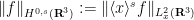
is the weighted norm

\displaystyle  \|f\|_{H^{0,s}({\bf R}^3)} := \| \langle x \rangle^s f \|_{L^2_x({\bf R}^3)}

and {\langle x \rangle := (1+|x|^2)^{1/2}}.

This principle allows one to extend the convergence (9) from test functions {f} to all functions in the weighted space {H^{0,1/2+\sigma}} by a density argument (though the radiation condition (8) has to be adapted suitably for this scale of spaces when doing so). The weighted space {H^{0,-1/2-\sigma}} on the left-hand side is optimal, as can be seen from the asymptotic (7); a duality argument similarly shows that the weighted space {H^{0,1/2+\sigma}} on the right-hand side is also optimal.

We prove this theorem below the fold. As observed long ago by Kato (and also reproduced below), this estimate is equivalent (via a Fourier transform in the spectral variable {\lambda}) to a useful estimate for the free Schrödinger equation known as the local smoothing estimate, which in particular implies the well-known RAGE theorem for that equation; it also has similar consequences for the free wave equation. As we shall see, it also encodes some spectral information about the Laplacian; for instance, it can be used to show that the Laplacian has no eigenvalues, resonances, or singular continuous spectrum. These spectral facts are already obvious from the Fourier transform representation of the Laplacian, but the point is that the limiting absorption principle also applies to more general operators for which the explicit diagonalisation afforded by the Fourier transform is not available. (Igor Rodnianski and I are working on a paper regarding this topic, of which I hope to say more about soon.)

In order to illustrate the main ideas and suppress technical details, I will be a little loose with some of the rigorous details of the arguments, and in particular will be manipulating limits and integrals at a somewhat formal level.

— 1. Uniqueness —

We first use an integration by parts argument to show uniqueness of the solution to the Helmholtz equation (6) assuming the radiation condition (8). For sake of concreteness we shall work with the sign {\pm=+}, and we will ignore issues of regularity, assuming all functions are as smooth as needed. (In practice, the elliptic nature of the Laplacian ensures that issues of regularity are easily dealt with.) If uniqueness fails, then by subtracting the two solutions, we obtain a non-trivial solution {u} to the homogeneous Helmholtz equation

\displaystyle  (-\Delta-\lambda) u = 0 \ \ \ \ \ (10)

such that

\displaystyle  u(x) = O(\frac{1}{|x|}); \quad (\partial_r - i\sqrt{\lambda}) u(x) = O( \frac{1}{|x|^2}).

Next, we introduce the charge current

\displaystyle  {\bf j}^i := \hbox{Im}( \overline{u} \partial^i u )

(using the usual Einstein index notations), and observe from (6) that this current is divergence-free:

\displaystyle  \partial_i {\bf j}^i = 0.

(This reflects the phase rotation invariance {u \mapsto e^{i\theta} u} of the equation (6), and can also be viewed as a version of the conservation of the Wronskian.) From Stokes’ theorem, and using polar coordinates, we conclude in particular that

\displaystyle  \int_{S^2} {\bf j}^r(r\omega)\ d\omega = 0

or in other words that

\displaystyle \int_{S^2} \hbox{Im}(\overline{u} \partial_r u)(r\omega)\ d\omega = 0.

Using the radiation condition, this implies in particular that

\displaystyle  \int_{S^2} |u(r\omega)|^2\ d\omega = O(r^{-3}) \ \ \ \ \ (11)

and

\displaystyle  \int_{S^2} |\partial_r u(r\omega)|^2\ d\omega = O(r^{-3}) \ \ \ \ \ (12)

as {r \rightarrow \infty}.

Now we use the “positive commutator method”. Consider the expression

\displaystyle  \int_{{\bf R}^3} [\partial_r, -\Delta-\lambda] u(x) \overline{u(x)}\ dx. \ \ \ \ \ (13)

(To be completely rigorous, one should insert a cutoff to a large ball, and then send the radius of that ball to infinity, in order to make the integral well-defined but we will ignore this technicality here.) On the one hand, we may integrate by parts (using (11), (12) to show that all boundary terms go to zero) and (10) to see that this expression vanishes. On the other hand, by expanding the Laplacian in polar coordinates we see that

\displaystyle  [-\Delta-\lambda, \partial_r] = -\frac{2}{r^2} \partial_r - \frac{2}{r^3} \Delta_\omega.

An integration by parts in polar coordinates (using (11), (12) to justify ignoring the boundary terms at infinity) shows that

\displaystyle  -\int_{{\bf R}^3} \frac{2}{r^2} \partial_r u(x) \overline{u(x)}\ dx = 8 \pi |u(0)|^2

and

\displaystyle  -\int_{{\bf R}^3} \frac{2}{r^3} \Delta_\omega u(x) \overline{u(x)}\ dx = 2 \int_{{\bf R}^3} \frac{|\nabla_{\hbox{ang}}| u(x)|^2}{|x|}\ dx

where {|\nabla_{\hbox{ang}} u(x)|^2 := |\nabla u(x)|^2 - |\partial_r u(x)|^2} is the angular part of the kinetic energy density {|\nabla u(x)|^2}. We obtain (a degenerate case of) the Pohazaev-Morawetz identity

\displaystyle  8 \pi |u(0)|^2 + 2 \int_{{\bf R}^3} \frac{|\nabla_{\hbox{ang}} u(x)|^2}{|x|}\ dx = 0

which implies in particular that {u} vanishes at the origin. Translating {u} around (noting that this does not affect either the Helmholtz equation or the Sommerfeld radiation condition) we see that {u} vanishes completely. (Alternatively, one can replace {\partial_r} by the smoothed out multiplier {\frac{x \cdot \nabla}{\langle x \rangle}}, in which case the Pohazaev-Morawetz identity acquires a term of the form {\int_{{\bf R}^3} \frac{|u(x)|^2}{\langle x \rangle^5}\ dx} which is enough to directly ensure that {u} vanishes.)

— 2. Proof of the limiting absorption principle —

We now sketch a proof of the limiting absorption principle, also based on the positive commutator method. For notational simplicity we shall only consider the case when {\lambda} is comparable to {1}, though the method we give here also yields the general case after some more bookkeeping.

Let {\sigma > 0} be a small exponent to be chosen later, and let {f} be normalised to have {H^{0,1/2+\sigma}({\bf R}^3)} norm equal to {1}. For sake of concreteness let us take the {+} sign, so that we wish to bound {u := R( \lambda + i \epsilon) f}. This {u} obeys the Helmholtz equation

\displaystyle  \Delta u + \lambda u = f - i \epsilon u. \ \ \ \ \ (14)

For positive {\epsilon}, we also see from the spectral theorem that {u} lies in {L^2({\bf R}^3)}; the bound here though depends on {\epsilon}, so we can only use this {L^2({\bf R}^3)} regularity for qualitative purposes (and specifically, for ensuring that boundary terms at infinity from integration by parts vanish) rather than quantitatively.

Once again, we may apply the positive commutator method. If we again consider the expression (13), then on the one hand this expression evaluates as before to

\displaystyle  8 \pi |u(0)|^2 + 2 \int_{{\bf R}^3} \frac{|\nabla_{\hbox{ang}} u(x)|^2}{|x|}\ dx.

On the other hand, integrating by parts using (14), this expression also evaluates to

\displaystyle  2 \hbox{Re} \int_{{\bf R}^3} (\partial_r (-f + i \epsilon u)) \overline{u}\ dx.

Integrating by parts and using Cauchy-Schwarz and the normalisation on {f} (and also Hardy’s inequality), we thus see that

\displaystyle  |u(0)|^2 + \int_{{\bf R}^3} \frac{|\nabla_{\hbox{ang}} u(x)|^2}{|x|}\ dx \lesssim \| u\|_{H^{0,-3/2-\sigma}} + \| \partial_r u \|_{H^{0,-1/2-\sigma}} + \epsilon \|u\|_{L^2} \|\nabla u\|_{L^2}.

A slight modification of this argument, replacing the operator {\partial_r} with the smoothed out variant

\displaystyle  (\frac{r}{\langle r \rangle} - \sigma \frac{r}{\langle r \rangle^{1+2\sigma}}) \partial_r

yields (after a tedious computation)

\displaystyle  \int_{{\bf R}^3} \frac{|u(x)|^2}{\langle x \rangle^{3+2\sigma}} + \frac{|\nabla u(x)|^2}{\langle x \rangle^{1+2\sigma}}\ dx \lesssim \| u\|_{H^{0,-3/2-\sigma}} + \| \partial_r u \|_{H^{0,-1/2-\sigma}} + \epsilon \|u\|_{L^2}^2.

The left-hand side is {\| u \|_{H^{0,-3/2-\sigma}}^2 + \| \nabla u \|_{H^{0,-1/2-\sigma}}^2}; we can thus absorb the first two terms of the right-hand side onto the left-hand side, leading one with

\displaystyle  \| u \|_{H^{0,-3/2-\sigma}}^2 + \| \nabla u \|_{H^{0,-1/2-\sigma}}^2 \lesssim \epsilon \| u \|_{L^2} \| \nabla u \|_{L^2}.

On the other hand, by taking the inner product of (14) against {iu} and using the self-adjointness of {\Delta+\lambda}, one has

\displaystyle  0 = \int_{{\bf R}^3} f \overline{iu} - \epsilon \int_{{\bf R}^3} |u|^2

and hence by Cauchy-Schwarz and the normalisation of {f}

\displaystyle  \epsilon \|u\|_{L^2}^2 \leq \|u\|_{H^{0,-1/2-\sigma}}.

Elliptic regularity estimates using (14) (together with the hypothesis that {\lambda} is comparable to {1}) also show that

\displaystyle  \| u \|_{H^{0,-1/2-\sigma}} \lesssim \| \nabla u \|_{H^{0,-1/2-\sigma}} + 1

and

\displaystyle  \| \nabla u \|_{L^2} \lesssim \| u \|_{L^2} + 1;

putting all these estimates together, we obtain

\displaystyle  \| u \|_{H^{0,-1/2-\sigma}} \lesssim 1

as required.

Remark 2 In applications it is worth noting some additional estimates that can be obtained by variants of the above method (i.e. lots of integration by parts and Cauchy-Schwarz). From the Pohazaev-Morawetz identity, for instance, we can show some additional decay for the angular derivative:

\displaystyle  \| |\nabla_{\hbox{ang}} u| \|_{H^{0,-1/2}} \lesssim \|f\|_{H^{0,1/2+\sigma}}.

With the positive sign {\pm = +}, we also have the Sommerfeld type outward radiation condition

\displaystyle  \| \partial_r u - i \sqrt{\lambda} u \|_{H^{0,-1/2+\sigma}} \lesssim \|f\|_{H^{0,1/2+\sigma}}

if {\sigma > 0} is small enough. For the negative sign {\pm = -}, we have the inward radiating condition

\displaystyle  \| \partial_r u + i \sqrt{\lambda} u \|_{H^{0,-1/2+\sigma}} \lesssim \|f\|_{H^{0,1/2+\sigma}}

— 3. Spectral applications —

The limiting absorption principle can be used to deduce various basic facts about the spectrum of the Laplacian. For instance:

Proposition 2 (Purely absolutely continuous spectrum) As an operator on {L^2({\bf R}^3)}, {-\Delta} has only purely absolutely continuous spectrum on any compact subinterval {[a,b]} of {(0,+\infty)}.

Proof: (Sketch) By density, it suffices to show that for any test function {f \in C^\infty_0({\bf R}^3)}, the spectral measure {\mu_f} of {-\Delta} relative to {f} is purely absolutely continuous on {[a,b]}. In view of (5), we have

\displaystyle  \mu_f = \lim_{\epsilon \rightarrow 0^+} \frac{1}{\pi} \hbox{Im} \langle R(\cdot+i\epsilon) f, f \rangle

in the sense of distributions, so from Fatou’s lemma it suffices to show that {\hbox{Im} \langle R(\cdot+i\epsilon) f, f \rangle} is uniformly bounded on {[a,b]}, uniformly in {\epsilon}. But this follows from the limiting absorption principle and Cauchy-Schwarz. \Box

Remark 3 The Laplacian {-\Delta} also has no (point) spectrum at zero or negative energies, but this cannot be shown purely from the limiting absorption principle; if one allows a non-zero potential, then the limiting absorption principle holds (assuming suitable “short-range” hypotheses on the potential) but (as is well known in quantum mechanics) one can have eigenvalues (bound states) at zero or negative energies.

— 4. Local smoothing —

Another key application of the limiting absorption principle is to obtain local smoothing estimates for both the Schrödinger and wave equations. Here is an instance of local smoothing for the Schrödinger equation:

Theorem 3 (Homogeneous local smoothing for Schrödinger) If {f \in L^2({\bf R}^3)}, and {u: {\bf R} \times {\bf R}^3 \rightarrow {\bf C}} is the (tempered distributional) solution to the homogeneous Schrödinger equation {i u_t + \Delta u = 0}, {u(0)=f} (or equivalently, {u(t) = e^{it\Delta} f}), then one has

\displaystyle  \| |\nabla|^{1/2} u \|_{L^2_t H^{0,-1/2-\sigma}_x({\bf R} \times {\bf R}^3)} \lesssim \| f \|_{L^2({\bf R}^3)}

for any fixed {\sigma > 0}.

The {|\nabla|^{1/2}} factor in this estimate is the “smoothing” part of the local smoothing estimate, while the negative weight {-1/2-\sigma} is the “local” part. There is also a version of this local smoothing estimate for the inhomogeneous Schrödinger equation {i u_t + \Delta u = F} which is in fact essentially equivalent to the limiting absorption principle (as observed by Kato), which we will not give here.

Proof: We begin by using the {TT^*} method. By duality, the claim is equivalent to

\displaystyle  \| |\nabla|^{1/2} \int_{\bf R} e^{-it\Delta} F(t)\ dt \|_{L^2({\bf R}^3)} \lesssim \| F \|_{L^2_t H^{0,1/2+\sigma}_x({\bf R} \times {\bf R}^3)}

which by squaring is equivalent to

\displaystyle  \| |\nabla| \int_{\bf R} e^{i(t-t')\Delta} F(t')\ dt' \|_{L^2_t H^{0,-1/2-\sigma}_x({\bf R} \times {\bf R}^3)} \lesssim \| F \|_{L^2_t H^{0,1/2+\sigma}_x({\bf R} \times {\bf R}^3)}. \ \ \ \ \ (15)

From (5) one has (formally, at least)

\displaystyle  e^{it\Delta} = \lim_{\epsilon \rightarrow 0^+} \frac{1}{\pi} \int_{\bf R} (\hbox{Im} R(y+i\epsilon)) e^{-ity}\ dy.

Because {-\Delta} only has spectrum on the positive real axis, {\hbox{Im} R(y+i0)} vanishes on the negative real axis, and so (after carefully dealing with the contribution near the zero energy) one has

\displaystyle  e^{it\Delta} = \lim_{\epsilon \rightarrow 0^+} \frac{1}{\pi} \int_0^\infty (\hbox{Im} R(y+i\epsilon)) e^{-ity}\ dy.

Taking the time-Fourier transform

\displaystyle  \hat F(y) := \int_{\bf R} e^{ity} F(t)

we thus have

\displaystyle  \int_{\bf R} e^{i(t-t')\Delta} F(t')\ dt' = \lim_{\epsilon \rightarrow 0^+} \frac{1}{\pi} \int_{\bf R} e^{-ity} (\hbox{Im} R(y+i\epsilon)) \hat F(y)\ dy.

Applying Plancherel’s theorem and Fatou’s lemma (and commuting the {L^2_t} and {H^{0,-1/2-\sigma}_x} norms), we can bound the LHS of (15) by

\displaystyle  \lesssim \| |\nabla| (\hbox{Im} R(y+i\epsilon)) \hat F(y) \|_{L^2_y H^{0,-1/2-\sigma}_x({\bf R} \times {\bf R}^3)}

while the right-hand side is comparable to

\displaystyle  \lesssim \| \hat F(y) \|_{L^2_y H^{0,1/2+\sigma}_x({\bf R} \times {\bf R}^3)}.

The claim now follows from the limiting absorption principle (and elliptic regularity). \Box

Remark 4 The above estimate was proven by taking a Fourier transform in time, and then applying the limiting absorption principle, which was in turn proven by using the positive commutator method. An equivalent way to proceed is to establish the local smoothing estimate directly by the analogue of the positive commutator method for Schrödinger flows, namely Morawetz multiplier method in which one contracts the stress-energy tensor (or variants thereof) against well-chosen vector fields, and integrates by parts.

An analogous claim holds for solutions to the wave equation

\displaystyle  -\partial_t^2 u + \Delta u = 0

with initial data {u(0)= u_0}, {\partial_t u(0) = u_1}, with the relevant estimate being that

\displaystyle  \| |\nabla_{t,x} u| \|_{L^2_t H^{0,-1/2-\sigma}({\bf R} \times {\bf R}^3)} \lesssim \| u_0 \|_{H^1({\bf R}^3)} + \| u_1 \|_{L^2({\bf R}^3)}.

As before, this estimate can also be proven directly using the Morawetz multiplier method.

— 5. The RAGE theorem —

Another consequence of limiting absorption, closely related both to absolutely continuous spectrum and to local smoothing, is the RAGE theorem (named after Ruelle, Amrein, Georgescu, and Enss), specialised to the free Schrödinger equation:

Theorem 4 (RAGE for Schrödinger) If {f \in L^2({\bf R}^3)}, and {K} is a compact subset of {{\bf R}^3}, then {\|e^{it\Delta} f \|_{L^2(K)} \rightarrow 0} as {t \rightarrow \pm \infty}.

Proof: By a density argument we may assume that {f} lies in, say, {H^2({\bf R}^3)}. Then {e^{it\Delta} f} is uniformly bounded in {H^2({\bf R}^3)}, and is Lipschitz in time in the {L^2({\bf R}^3)} (and hence {L^2(K)}) norm. On the other hand, from local smoothing we know that {\int_T^{T+1} \|e^{it\Delta}\|_{L^2(K)}\ dt} goes to zero as {T \rightarrow \pm \infty}. Putting the two facts together we obtain the claim. \Box

Remark 5 One can also deduce this theorem from the fact that {-\Delta} has purely absolutely continuous spectrum, using the abstract form of the RAGE theorem due to the authors listed above (which can be thought of as a Hilbert space-valued version of the Riemann-Lebesgue lemma).

There is also a similar RAGE theorem for the wave equation (with {L^2} replaced by the energy space {H^1 \times L^2}) whose precise statement we omit here.

— 6. The limiting amplitude principle —

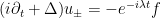
A close cousin to the limiting absorption principle, which governs the limiting behaviour of the resolvent as it approaches the spectrum, is the limiting amplitude principle, which governs the asymptotic behaviour of a Schrödinger or wave equation with oscillating forcing term. We give this principle for the Schrödinger equation (the case for the wave equation is analogous):

Theorem 5 (Limiting amplitude principle) Let {f \in L^2({\bf R}^3)} be compactly supported, let {\mu > 0}, and let {u} be a solution to the forced Schrödinger equation {iu_t + \Delta u = e^{-i\mu t} f} which lies in {L^2({\bf R}^3)} at time zero. Then for any compact set {K}, {e^{i\mu T} u} converges in {L^2(K)} as {T \rightarrow +\infty} to {v}, the solution to the Helmholtz equation {\Delta v + \mu v = f} obeying the outgoing radiation condition (7).

Proof: (Sketch) By subtracting off the free solution {e^{it\Delta} u(0)} (which decays in {L^2(K)} by the RAGE theorem), we may assume that {u(0)=0}. From the Duhamel formula we then have

\displaystyle  u(T) = -i \int_0^T e^{i (T-t) \Delta} e^{-i\mu t} f\ dt

and thus (after changing variables from {t} to {T-t})

\displaystyle  e^{i\mu T} u(T) = - i \int_0^T e^{it(\Delta+\mu)} f\ dt.

We write the right-hand side as

\displaystyle  - i \lim_{\epsilon \rightarrow 0^+} \int_0^T e^{it(\Delta+\mu+i\epsilon)} f\ dt.

From the limiting absorption principle, the integral {-i \int_0^\infty e^{it(\Delta+\mu+i\epsilon)} f\ dt} converges to {v}, and so it suffices to show that the expression

\displaystyle  \lim_{\epsilon \rightarrow 0^+} \int_T^\infty e^{it(\Delta+\mu+i\epsilon)} f\ dt

converges to zero as {T \rightarrow +\infty} in {L^2(K)} norm. Evaluating the integral, we are left with showing that

\displaystyle  \lim_{\epsilon \rightarrow 0^+} e^{iT\Delta} R(\mu+i\epsilon) f

converges to zero as {T \rightarrow +\infty} in {L^2(K)} norm.

By using contour integration, one can write

\displaystyle  \lim_{\epsilon \rightarrow 0^+} e^{iT\Delta} R(\mu+i\epsilon) f = \frac{1}{2\pi i} \lim_{\epsilon \rightarrow 0^+} \lim_{\epsilon' \rightarrow 0^+} \int_{\bf R} \frac{e^{-iTx}}{x-\mu-i\epsilon} R(x+i\epsilon') f\ dx.

On the other hand, from the explicit solution for the resolvent (and the compact support of {f}), {R(x+i\epsilon') f} can be shown to vary in a Hölder continuous fashion on {x} in the {L^2(K)} norm (uniformly in {x, \epsilon'}), and to decay at a polynomial rate as {x \rightarrow \pm \infty}. Since

\displaystyle  \int_{\bf R} \frac{e^{-iTx}}{x-\mu-i\epsilon}\ dx = 0

for {T>0}, the required decay in {L^2(K)} then follows from a routine calculation. \Box

Remark 6 More abstractly, it was observed by Eidus that the limiting amplitude principle for a general Schrödinger or wave equation can be deduced from the limiting absorption principle and a Hölder continuity bound on the resolvent.