Lars Hörmander, who made fundamental contributions to all areas of partial differential equations, but particularly in developing the analysis of variable-coefficient linear PDE, died last Sunday, aged 81.
I unfortunately never met Hörmander personally, but of course I encountered his work all the time while working in PDE. One of his major contributions to the subject was to systematically develop the calculus of Fourier integral operators (FIOs), which are a substantial generalisation of pseudodifferential operators and which can be used to (approximately) solve linear partial differential equations, or to transform such equations into a more convenient form. Roughly speaking, Fourier integral operators are to linear PDE as canonical transformations are to Hamiltonian mechanics (and one can in fact view FIOs as a quantisation of a canonical transformation). They are a large class of transformations, for instance the Fourier transform, pseudodifferential operators, and smooth changes of the spatial variable are all examples of FIOs, and (as long as certain singular situations are avoided) the composition of two FIOs is again an FIO.
The full theory of FIOs is quite extensive, occupying the entire final volume of Hormander’s famous four-volume series “The Analysis of Linear Partial Differential Operators”. I am certainly not going to try to attempt to summarise it here, but I thought I would try to motivate how these operators arise when trying to transform functions. For simplicity we will work with functions  on a Euclidean domain
  (although FIOs can certainly be defined on more general smooth manifolds, and there is an extension of the theory that also works on manifolds with boundary). As this will be a heuristic discussion, we will ignore all the (technical, but important) issues of smoothness or convergence with regards to the functions, integrals and limits that appear below, and be rather vague with terms such as “decaying” or “concentrated”.
A function can be viewed from many different perspectives (reflecting the variety of bases, or approximate bases, that the Hilbert space  offers). Most directly, we have the physical space perspective, viewing
  as a function
  of the physical variable
  . In many cases, this function will be concentrated in some subregion
  of physical space. For instance, a gaussian wave packet

where  ,
,  and
and  are parameters, would be physically concentrated in the ball
  . Then we have the frequency space (or momentum space) perspective, viewing now as a function
  of the frequency variable
  . For this discussion, it will be convenient to normalise the Fourier transform using a small constant (which has the physical interpretation of Planck’s constant if one is doing quantum mechanics), thus

For instance, for the gaussian wave packet (1), one has

and so we see that is concentrated in frequency space in the ball  .
.
However, there is a third (but less rigorous) way to view a function in , which is the phase space perspective in which one tries to view as distributed simultaneously in physical space and in frequency space, thus being something like a measure on the phase space  . Thus, for instance, the function (1) should heuristically be concentrated on the region
  in phase space. Unfortunately, due to the uncertainty principle, there is no completely satisfactory way to canonically and rigorously define what the “phase space portrait” of a function should be. (For instance, the Wigner transform of can be viewed as an attempt to describe the distribution of the
  energy of in phase space, except that this transform can take negative or even complex values; see Folland’s book for further discussion.) Still, it is a very useful heuristic to think of functions has having a phase space portrait, which is something like a non-negative measure on phase space that captures the distribution of functions in both space and frequency, albeit with some “quantum fuzziness” that shows up whenever one tries to inspect this measure at scales of physical space and frequency space that together violate the uncertainty principle. (The score of a piece of music is a good everyday example of a phase space portrait of a function, in this case a sound wave; here, the physical space is the time axis (the horizontal dimension of the score) and the frequency space is the vertical dimension. Here, the time and frequency scales involved are well above the uncertainty principle limit (a typical note lasts many hundreds of cycles, whereas the uncertainty principle kicks in at
  cycles) and so there is no obstruction here to musical notation being unambiguous.) Furthermore, if one takes certain asymptotic limits, one can recover a precise notion of a phase space portrait; for instance if one takes the semiclassical limit
  then, under certain circumstances, the phase space portrait converges to a well-defined classical probability measure on phase space; closely related to this is the high frequency limit of a fixed function, which among other things defines the wave front set of that function, which can be viewed as another asymptotic realisation of the phase space portrait concept.
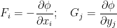
If functions in can be viewed as a sort of distribution in phase space, then linear operators  should be viewed as various transformations on such distributions on phase space. For instance, a pseudodifferential operator
  should correspond (as a zeroth approximation) to multiplying a phase space distribution by the symbol
  of that operator, as discussed in this previous blog post. Note that such operators only change the amplitude of the phase space distribution, but not the support of that distribution.
Now we turn to operators that alter the support of a phase space distribution, rather than the amplitude; we will focus on unitary operators to emphasise the amplitude preservation aspect. These will eventually be key examples of Fourier integral operators. A physical translation 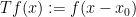 should correspond to pushing forward the distribution by the transformation
  , as can be seen by comparing the physical and frequency space supports of
  with that of . Similarly, a frequency modulation
 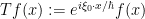 should correspond to the transformation
 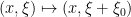 ; a linear change of variables
  , where
  is an invertible linear transformation, should correspond to
 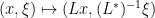 ; and finally, the Fourier transform
  should correspond to the transformation
 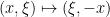 .
.
Based on these examples, one may hope that given any diffeomorphism  of phase space, one could associate some sort of unitary (or approximately unitary) operator
  , which (heuristically, at least) pushes the phase space portrait of a function forward by
  . However, there is an obstruction to doing so, which can be explained as follows. If
  pushes phase space portraits by , and pseudodifferential operators multiply phase space portraits by
  , then this suggests the intertwining relationship

and thus  is approximately conjugate to :

The formalisation of this fact in the theory of Fourier integral operators is known as Egorov’s theorem, due to Yu Egorov (and not to be confused with the more widely known theorem of Dmitri Egorov in measure theory).
Applying commutators, we conclude the approximate conjugacy relationship
![\displaystyle \frac{1}{i\hbar} [(a \circ \Phi)(X,D), (b \circ \Phi)(X,D)] \approx T_\Phi^{-1} \frac{1}{i\hbar} [a(X,D), b(X,D)] T_\Phi.](https://s0.wp.com/latex.php?latex=%5Cdisplaystyle++%5Cfrac%7B1%7D%7Bi%5Chbar%7D+%5B%28a+%5Ccirc+%5CPhi%29%28X%2CD%29%2C+%28b+%5Ccirc+%5CPhi%29%28X%2CD%29%5D+%5Capprox+T_%5CPhi%5E%7B-1%7D+%5Cfrac%7B1%7D%7Bi%5Chbar%7D+%5Ba%28X%2CD%29%2C+b%28X%2CD%29%5D+T_%5CPhi.&bg=ffffff&fg=000000&s=0&c=20201002)
Now, the pseudodifferential calculus (as discussed in this previous post) tells us (heuristically, at least) that
![\displaystyle \frac{1}{i\hbar} [a(X,D), b(X,D)] \approx \{ a, b \}(X,D)](https://s0.wp.com/latex.php?latex=%5Cdisplaystyle++%5Cfrac%7B1%7D%7Bi%5Chbar%7D+%5Ba%28X%2CD%29%2C+b%28X%2CD%29%5D+%5Capprox+%5C%7B+a%2C+b+%5C%7D%28X%2CD%29&bg=ffffff&fg=000000&s=0&c=20201002)
and
![\displaystyle \frac{1}{i\hbar} [(a \circ \Phi)(X,D), (b \circ \Phi)(X,D)] \approx \{ a \circ \Phi, b \circ \Phi \}(X,D)](https://s0.wp.com/latex.php?latex=%5Cdisplaystyle++%5Cfrac%7B1%7D%7Bi%5Chbar%7D+%5B%28a+%5Ccirc+%5CPhi%29%28X%2CD%29%2C+%28b+%5Ccirc+%5CPhi%29%28X%2CD%29%5D+%5Capprox+%5C%7B+a+%5Ccirc+%5CPhi%2C+b+%5Ccirc+%5CPhi+%5C%7D%28X%2CD%29&bg=ffffff&fg=000000&s=0&c=20201002)
where  is the Poisson bracket. Comparing this with (2), we are then led to the compatibility condition

thus needs to preserve (approximately, at least) the Poisson bracket, or equivalently needs to be a symplectomorphism (again, approximately at least).
Now suppose that is a symplectomorphism. This is morally equivalent to the graph  being a Lagrangian submanifold of
  (where we give the second copy of phase space the negative
  of the usual symplectic form
  , thus yielding
  as the full symplectic form on ; this is another instantiation of the closed graph theorem, as mentioned in this previous post. This graph is known as the canonical relation for the (putative) FIO that is associated to . To understand what it means for this graph to be Lagrangian, we coordinatise as
  suppose temporarily that this graph was (locally, at least) a smooth graph in the
  and
and  variables, thus

for some smooth functions  . A brief computation shows that the Lagrangian property of
  is then equivalent to the compatibility conditions


for  , where
  denote the components of
  . Some Fourier analysis (or Hodge theory) lets us solve these equations as
for some smooth potential function  . Thus, we have parameterised our graph as

so that maps 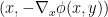 to
to  .
.
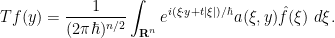
A reasonable candidate for an operator associated to and in this fashion is the oscillatory integral operator
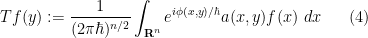
for some smooth amplitude function (note that the Fourier transform is the special case when  and
and  , which helps explain the genesis of the term “Fourier integral operator”). Indeed, if one computes an inner product
 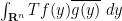 for gaussian wave packets
  of the form (1) and localised in phase space near
 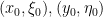 respectively, then a Taylor expansion of
  around
  , followed by a stationary phase computation, shows (again heuristically, and assuming is suitably non-degenerate) that
  has (3) as its canonical relation. (Furthermore, a refinement of this stationary phase calculation suggests that if is normalised to be the half-density
  , then should be approximately unitary.) As such, we view (4) as an example of a Fourier integral operator (assuming various smoothness and non-degeneracy hypotheses on the phase and amplitude which we do not detail here).
Of course, it may be the case that is not a graph in the  coordinates (for instance, the key examples of translation, modulation, and dilation are not of this form), but then it is often a graph in some other pair of coordinates, such as
  . In that case one can compose the oscillatory integral construction given above with a Fourier transform, giving another class of FIOs of the form
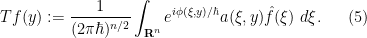
This class of FIOs covers many important cases; for instance, the translation, modulation, and dilation operators considered earlier can be written in this form after some Fourier analysis. Another typical example is the half-wave propagator  for some time
  , which can be written in the form
This corresponds to the phase space transformation 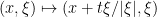 , which can be viewed as the classical propagator associated to the “quantum” propagator
  . More generally, propagators for linear Hamiltonian partial differential equations can often be expressed (at least approximately) by Fourier integral operators corresponding to the propagator of the associated classical Hamiltonian flow associated to the symbol of the Hamiltonian operator
  ; this leads to an important mathematical formalisation of the correspondence principle between quantum mechanics and classical mechanics, that is one of the foundations of microlocal analysis and which was extensively developed in Hörmander’s work. (More recently, numerically stable versions of this theory have been developed to allow for rapid and accurate numerical solutions to various linear PDE, for instance through Emmanuel Candés’ theory of curvelets, so the theory that Hörmander built now has some quite significant practical applications in areas such as geology.)
In some cases, the canonical relation may have some singularities (such as fold singularities) which prevent it from being written as graphs in the previous senses, but the theory for defining FIOs even in these cases, and in developing their calculus, is now well established, in large part due to the foundational work of Hörmander.


10 comments
Comments feed for this article
30 November, 2012 at 12:45 pm
Marcelo de Almeida
\beign{equation} (a \circ \Phi)(X,D) \approx T_\Phi^{-1} a(X,D) T_\Phi
Should be
\begin{equation} (a \circ \Phi)(X,D) \approx T_\Phi^{-1} a(X,D) T_\Phi\end{equation}
[Corrected, thanks – T.]
1 December, 2012 at 2:06 am
Maurice de Gosson
The discussion of the phase space properties of the FIOs and PDOs is very approximative. The operators T are the generators of the metaplectic group; this has to be explained, because symplectic/metaplectic covariance is one crucial property leading to Weyl operators (it is a characteristic property). Otherwise, interesting popular mathematics! Hörmander was indeed a great man. His contributions toi the theory of functions of complex variables is also far from being negligible.
2 December, 2012 at 6:38 pm
John
Dear terry,
I am not sure I understood the music score analogy completely, in particular how one defines the corresponding notion of uncertainty principle. What did you mean by cycles? And why would O(1) number of cycles for one note be a problem? Thx
2 December, 2012 at 7:55 pm
Terence Tao
A musical note can be viewed as a rectangle in phase space (though in a musical score, it is depicted instead as an oval), with the horizontal extent of the rectangle describing the duration of the note, and the vertical extent describing the frequency range. Note that the vertical extent is non-zero (unless the note is a pure sinusoidal wave that lasts forever). The uncertainty principle asserts that the product of the horizontal extent (measured in seconds) and the vertical extent (measured in Hertz) has to be >> 1.
In a musical scale, going one octave up corresponds to multiplying the frequency by 2; there are twelve tones in an octave, so (assuming equal temperament) adjacent notes in a scale differ by a multiplicative factor of (each note has 6% higher frequency than the previous one). To distinguish adjacent notes from each other, one thus needs a frequency uncertainty of less than 6% of the frequency of the note, which by the uncertainty principle corresponds to a minimum of about 17 cycles for the time uncertainty. (For middle C, for instance, which has a frequency of 260 Hz, this is about 0.06 seconds; of course, actual musical notes last far longer than this and so there is no obstruction from the uncertainty principle with discerning notes from each other. But if one played a middle C and a middle C# note, for instance, for less than 0.06 seconds each, the two notes would basically be indistinguishable from each other (they would make the same number of complete cycles in that time period).
11 September, 2014 at 6:21 am
Christian
Right after the last equation, shouldn’t it be: (x,\xi) \mapsto (x + t \frac{\xi}{ \vert \xi \vert , \xi ) instead of (x,\xi) \mapsto (x + t \vert \xi \vert , \xi ). At least this would be the associated Hamiltonian flow.
Thanks for the nice article!
[Corrected, thanks – T.]
4 September, 2015 at 1:22 am
Moritz
You indicated that there is are fourier integral operators for manifolds with boundary. Could you give a reference to that? Thank you.
11 October, 2015 at 1:45 am
Lars Hörmander » kryakin_y
[…] Юноша с горящим взглядом. Ушел. Прочитал у солнечного Тао де […]
27 November, 2015 at 6:53 am
Lars Hörmander | yuriy_kryakin
[…] Юноша с горящим взглядом. Ушел. Прочитал у солнечного Тао де […]
24 January, 2016 at 5:15 am
Matemáticos de la Historia :: Lars Hörmander | María de los Milagros Langhi :: Blog personal
[…] https://terrytao.wordpress.com/2012/11/30/lars-hormander/ […]
17 June, 2017 at 1:15 pm
Lars Hörmander | kryakin_f
[…] Юноша с горящим взглядом. Ушел. Прочитал у солнечного Тао де […]