One of the basic problems in the field of operator algebras is to develop a functional calculus for either a single operator  , or a collection
  of operators. These operators could in principle act on any function space, but typically one either considers complex matrices (which act on a complex finite dimensional space), or operators (either bounded or unbounded) on a complex Hilbert space. (One can of course also obtain analogous results for real operators, but we will work throughout with complex operators in this post.)
Roughly speaking, a functional calculus is a way to assign an operator  or
or  to any function
  in a suitable function space, which is linear over the complex numbers, preserve the scalars (i.e.
  when
when  ), and should be either an exact or approximate homomorphism in the sense that

should hold either exactly or approximately. In the case when the  are self-adjoint operators acting on a Hilbert space (or Hermitian matrices), one often also desires the identity

to also hold either exactly or approximately. (Note that one cannot reasonably expect (1) and (2) to hold exactly for all  if the
  and their adjoints
  do not commute with each other, so in those cases one has to be willing to allow some error terms in the above wish list of properties of the calculus.) Ideally, one should also be able to relate the operator norm of
  or
or  with something like the uniform norm on
  . In principle, the existence of a good functional calculus allows one to manipulate operators as if they were scalars (or at least approximately as if they were scalars), which is very helpful for a number of applications, such as partial differential equations, spectral theory, noncommutative probability, and semiclassical mechanics. A functional calculus for multiple operators can be particularly valuable as it allows one to treat as being exact or approximate scalars simultaneously. For instance, if one is trying to solve a linear differential equation that can (formally at least) be expressed in the form
for some data , unknown function  , some differential operators
  , and some nice function , then if one’s functional calculus is good enough (and is suitably “elliptic” in the sense that it does not vanish or otherwise degenerate too often), one should be able to solve this equation either exactly or approximately by the formula

which is of course how one would solve this equation if one pretended that the operators were in fact scalars. Formalising this calculus rigorously leads to the theory of pseudodifferential operators, which allows one to (approximately) solve or at least simplify a much wider range of differential equations than one what can achieve with more elementary algebraic transformations (e.g. integrating factors, change of variables, variation of parameters, etc.). In quantum mechanics, a functional calculus that allows one to treat operators as if they were approximately scalar can be used to rigorously justify the correspondence principle in physics, namely that the predictions of quantum mechanics approximate that of classical mechanics in the semiclassical limit  .
.
There is no universal functional calculus that works in all situations; the strongest functional calculi, which are close to being an exact *-homomorphisms on very large class of functions, tend to only work for under very restrictive hypotheses on or (in particular, when  , one needs the to commute either exactly, or very close to exactly), while there are weaker functional calculi which have fewer nice properties and only work for a very small class of functions, but can be applied to quite general operators or . In some cases the functional calculus is only formal, in the sense that or has to be interpreted as an infinite formal series that does not converge in a traditional sense. Also, when one wishes to select a functional calculus on non-commuting operators , there is a certain amount of non-uniqueness: one generally has a number of slightly different functional calculi to choose from, which generally have the same properties but differ in some minor technical details (particularly with regards to the behaviour of “lower order” components of the calculus). This is a similar to how one has a variety of slightly different coordinate systems available to parameterise a Riemannian manifold or Lie group. This is on contrast to the
  case when the underlying operator
  is (essentially) normal (so that commutes with
  ); in this special case (which includes the important subcases when is unitary or (essentially) self-adjoint), spectral theory gives us a canonical and very powerful functional calculus which can be used without further modification in applications.
Despite this lack of uniqueness, there is one standard choice for a functional calculus available for general operators , namely the Weyl functional calculus; it is analogous in some ways to normal coordinates for Riemannian manifolds, or exponential coordinates of the first kind for Lie groups, in that it treats lower order terms in a reasonably nice fashion. (But it is important to keep in mind that, like its analogues in Riemannian geometry or Lie theory, there will be some instances in which the Weyl calculus is not the optimal calculus to use for the application at hand.)
I decided to write some notes on the Weyl functional calculus (also known as Weyl quantisation), and to sketch the applications of this calculus both to the theory of pseudodifferential operators. They are mostly for my own benefit (so that I won’t have to redo these particular calculations again), but perhaps they will also be of interest to some readers here. (Of course, this material is also covered in many other places. e.g. Folland’s “harmonic analysis in phase space“.)
— 1. Weyl quantisation of polynomials —
The simplest class of functions to which one can set up a functional calculus are the polynomials, as this does not require any analytic tools to define. To begin with we will ignore the conjugation structure, thus we will not attempt to implement (2).
In order to be able to freely compose all the operators under consideration, we will assume that there is some dense space of test functions (or perhaps Schwartz functions) which is preserved by all of the , so that any composition of finitely many of the will be densely defined. (Alternatively, one could proceed at a purely formal level for this discussion, working in an abstract algebra generated by the .)
In the case of a single operator , the polynomial calculus is obvious: given any polynomial

with complex coefficients  , one can define to be the operator

In other words, the functional calculus  is the linear map that takes each monomial
  to the operator
  . This calculus is of course an exact homomorphism, as it is linear and obeys (1) exactly.
Now we consider the situation with multiple operators. For simplicity, let us just consider the case of two operators  . We then consider a polynomial
with complex coefficients  , and ask how to define the operator
  .
.
The most obvious way to define is by direct substitution, which I will call the Kohn-Nirenberg calculus:

(Depending on the interpretation of the operators , this calculus might also be referred to as the Wick-ordered calculus or normal-ordered calculus.) This is certainly a well-defined calculus, but when and  do not commute, the calculus has a bias in that it always places to the left of ; in particular, if one interchanges the roles of
  and
and  then one obtains a different calculus, which one might call the anti-Kohn-Nirenberg calculus:
Intermediate, and more symmetric, between these two calculi, is the Weyl calculus
where the Weyl ordering  of the monomial
  is defined to be the average of all the
  ways to multiply
  copies of and
  copies of together:

where  range over all tuples which contain copies of and copies of , thus for instance
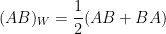

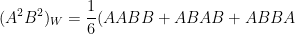

and so forth.
Remark 1 Strictly speaking, the use of the terminology here is an abuse of notation, because it suggests a functional relationship between and which need not be the case. In particular, if the monomials and  are equal as operators, this does not necessarily imply that the Weyl-ordered monomials and
  are equal. One could fix this notation by working first with formal symbols
  generating a free commutative algebra, and writing
  in place of , so that the Weyl map
  becomes a not-quite-homomorphism from the commutative algebra generated by
  and
and  to the non-commutative algebra generated by and . We have chosen however to not be quite so formal, and allow some abuse of notation to simplify the exposition.
When and commute, of course, all these calculi coincide with each other; it is only in the non-commuting case that some distinctions between the calculi emerge. The Weyl calculus may seem complicated, but it has somewhat cleaner formulae with regard to products. For instance, the Weyl calculus works perfectly with respect to powers  of affine combinations
  of , where
  are scalars:

(By this equation, we mean that if is the polynomial  , then
  is the operator
  .) Thus for instance


In contrast, the Kohn-Nirenberg calculus (or the anti-Kohn-Nirenberg calculus) distorts this ordering, for instance we have

Indeed, by comparing coefficients in (3) and using linearity we see that the identity (3) (for arbitrary  ) in fact uniquely defines the Weyl calculus. One consequence of this is that the Weyl calculus is not only symmetric with respect to interchange of the underlying operators , but in fact respects all linear changes of variable: if
  are scalar affine combinations of ,
  is a polynomial of two variables, and is the polynomial
  , then we have that

Indeed, from (3) we see that this identity holds for the mixed monomials  , and then by linearity it is true for all polynomials.
One can also extend the Weyl calculus to formal (i.e. not necessarily convergent) infinite series

by declaring to be the formal series of operators
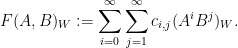
In doing so, the identity (3) can be expressed in a very convenient form

where we view the exponential function  here as the formal infinite series

Remark 2 The fact that Weyl calculus preserves the exponential map is the reason why we view this calculus as being analogous to normal coordinates in Riemannian geometry, as well as exponential coordinates (of the first kind) on Lie groups, discussed for instance in this previous blog post. In contrast, the Kohn-Nirenberg quantisation gives

which is analogous to exponential coordinates of the second kind on Lie groups.
Now we study the extent to which the homomorphism property (1) holds in the Weyl calculus, i.e. we study the discrepancy between  and
and  . When and commute, it is easy to see that (1) holds exactly. In general, these two expressions can be quite different; but when and almost commute, so that the commutator
 ![{[A,B] = AB-BA}](https://s0.wp.com/latex.php?latex=%7B%5BA%2CB%5D+%3D+AB-BA%7D&bg=ffffff&fg=000000&s=0&c=20201002) is non-zero but small, we expect (1) to be approximately true. Motivated by quantum-mechanical examples, we will study a model case when and obey the Heisenberg commutator relationship
is non-zero but small, we expect (1) to be approximately true. Motivated by quantum-mechanical examples, we will study a model case when and obey the Heisenberg commutator relationship
![\displaystyle [A,B] = i\hbar \ \ \ \ \ (6)](https://s0.wp.com/latex.php?latex=%5Cdisplaystyle++%5BA%2CB%5D+%3D+i%5Chbar+%5C+%5C+%5C+%5C+%5C+%286%29&bg=ffffff&fg=000000&s=0&c=20201002)
where  is a small positive real number. (In some literature, the sign convention here is reversed.) In this case, we see that any two ways to multiply copies of and
  copies of together will differ by polynomials of degree strictly less than
  . Among other things, this shows that any polynomial of and can be rewritten into a Weyl-ordered form, by first ordering the top degree terms (at the cost of introducing some messy lower degree terms) and then recursively working on the lower order terms. The same procedure also implies that this Weyl-ordered form is unique. For instance,
![\displaystyle AB = (AB)_W -\frac{1}{2}[A,B] = (AB - \frac{1}{2} i\hbar)_W.](https://s0.wp.com/latex.php?latex=%5Cdisplaystyle++AB+%3D+%28AB%29_W+-%5Cfrac%7B1%7D%7B2%7D%5BA%2CB%5D+%3D+%28AB+-+%5Cfrac%7B1%7D%7B2%7D+i%5Chbar%29_W.&bg=ffffff&fg=000000&s=0&c=20201002)
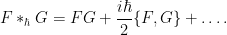
This already implies that for any two polynomials  , there must be a unique “product” polynomial
  with the property that

In the classical limit  , this operation is simply pointwise product:

Now we work out what the product operation  (known as the Moyal product) is for non-zero . To avoid some rather messy combinatorics, it turns out to be cleanest to proceed using the formal exponential function (5) applied to various combinations
  of and . (This is an instance of the method of generating functions in action.)
We first observe from (6) that we have the general commutation relationship
![\displaystyle [sA+tB, s'A+t'B] = i\hbar \omega( (s,t), (s',t') ) \ \ \ \ \ (8)](https://s0.wp.com/latex.php?latex=%5Cdisplaystyle++%5BsA%2BtB%2C+s%27A%2Bt%27B%5D+%3D+i%5Chbar+%5Comega%28+%28s%2Ct%29%2C+%28s%27%2Ct%27%29+%29+%5C+%5C+%5C+%5C+%5C+%288%29&bg=ffffff&fg=000000&s=0&c=20201002)
where  is the anti-symmetric form

This is already the first hint of the correspondence between quantum mechanics (whose dynamics is based on the commutator ![{\frac{i}{\hbar} [,]}](https://s0.wp.com/latex.php?latex=%7B%5Cfrac%7Bi%7D%7B%5Chbar%7D+%5B%2C%5D%7D&bg=ffffff&fg=000000&s=0&c=20201002) ) and classical mechanics (whose dynamics is based on the Poisson bracket
) and classical mechanics (whose dynamics is based on the Poisson bracket  ). From this and the Baker-Campbell-Hausdorff formula, we conclude (formally, at least) that


One can make this identity rigorous (at the level of formal power series) as follows. We first observe that the Hadamard lemma

holds at the level of formal power series, where  is the commutator operation
 ![{\hbox{ad}(X)(Y) := [X,Y]}](https://s0.wp.com/latex.php?latex=%7B%5Chbox%7Bad%7D%28X%29%28Y%29+%3A%3D+%5BX%2CY%5D%7D&bg=ffffff&fg=000000&s=0&c=20201002) . This can be seen by first establishing the formal differentiation identity
. This can be seen by first establishing the formal differentiation identity

(which comes from the formal identity  and the product rule) and then using this to solve for
  as a formal power series to conclude that

and then setting  . Using this lemma together with (8), we see in particular that

Now consider the expression

as a formal power series in  . Then
  is the identity, and the formal derivative
  can be expressed as


which after using (10) simplifies to

which on solving the formal series leads to

which gives (9) after setting  .
.
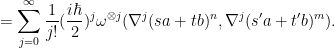
Combining (9), (5) and (7) (as well as the uniqueness of the Weyl ordering), we conclude that


where both sides are viewed as formal power series in indeterminates  . Comparing coefficients, we see that


with the convention that  vanishes for
  , and similarly for
  . We write

where  is the tensor product of copies of
  . Since

and similarly

where  denotes the gradient with respect to the variables, we conclude that
This formula is valid for all monomials 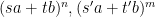 , and so by bilinearity we conclude the explicit formula

for the Moyal product, thus

The expression  is also known as the Poisson bracket of and
  , and is denoted
  , thus
Note that  is symmetric for even and anti-symmetric for odd . Subtracting, we conclude that

thus

Thus we see that the normalised commutator  of the Moyal product converges in the semiclassical limit ; this is one manifestation of the correspondence principle.
The above discussion was for two operators obeying the Heisenberg commutation relation (6), but one can check that a similar calculus can also be developed for any tuple of operators, and if they obey a Heisenberg-like commutation law
![\displaystyle [ \sum_{i=1}^k s_i A_i, \sum_{j=1}^k t_j A_j] = \omega( (s_1,\ldots,s_k), (t_1,\ldots,t_k) )](https://s0.wp.com/latex.php?latex=%5Cdisplaystyle++%5B+%5Csum_%7Bi%3D1%7D%5Ek+s_i+A_i%2C+%5Csum_%7Bj%3D1%7D%5Ek+t_j+A_j%5D+%3D+%5Comega%28+%28s_1%2C%5Cldots%2Cs_k%29%2C+%28t_1%2C%5Cldots%2Ct_k%29+%29&bg=ffffff&fg=000000&s=0&c=20201002)
for some anti-symmetric form  , then the Moyal product formula (11) holds; the arguments are basically identical to the two variable case (except for some notational complications) and are left as an exercise to the reader.
Once one has set up a calculus for complex polynomials  of some non-self-adjoint operators , one can then extend it to polynomials
  of the original arguments
  and their conjugates (or equivalently, to polynomials of the real and imaginary parts of the ) by using the calculus for
  . This allows one to define operators
  when
when  is a polynomial of the real and imaginary parts of , basically by substituting
  and
and  for
for  and
and  respectively. One advantage of the Weyl calculus, not shared in general by the Kohn-Nirenberg calculus, is that the identity (2) holds exactly; this is basically a special case of the affine invariance properties of the Weyl calculus mentioned earlier. In a similar vein, the Weyl calculus ensures that

for any complex polynomial , where  is the complex polynomial whose coefficients are the complex conjugates of the coefficients of . In particular, if are self-adjoint and has real coefficients, then
  is again self-adjoint.
— 2. Weyl quantisation of smooth symbols —
The above algebraic formalism allowed one to define the Weyl quantisation of any -tuple of operators (preserving some dense space of test functions) as long as was a polynomial; one could also handle the case when was a formal power series, provided that one was willing to make a formal power series also. But of course we would like to expand the calculus beyond the spaces of polynomials and formal power series.
One obvious way is to work with convergent power series instead of formal power series, but this approach, by definition, only applies for real analytic functions . Also, being real analytic (which, by the root test, can be viewed as an exponential decay hypothesis on the coefficients ) may not be enough in some cases to ensure convergence of the formal power series ; one may need faster decay on the (e.g. decay like  or something similar) before one can justify convergence in a suitable sense.
To get beyond the analytic category, it turns out that one can use Fourier-analytic methods, using Fourier expansions as a substitute for power series expansions. The key point, of course, is that Fourier analysis works well for spaces of functions that are significantly rougher than real analytic.
To illustrate the method, let us again work with just two operators and . We will assume that and are (essentially) self-adjoint, which by spectral theory suggests that one should be able to define for (sufficiently nice) real-valued functions  . (The distinction between real and complex functions was not apparent at the polynomial level, since any polynomial on a real vector space can be automatically complexified uniquely to a polynomial on the associated complex vector space.) The starting point is the Fourier inversion formula
where  is the Fourier transform, which in our choice of normalisations becomes

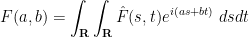
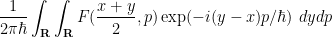
From the inversion formula, it is natural to expect that the Weyl quantisation of should be given by the formula

which in view of (5) leads us to
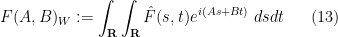
which we will take as a definition of for general functions .
Of course, to make this definition rigorous, one has to specify some regularity hypotheses on , and check that the integral actually converges in some suitable sense; also, it would be reassuring to verify that the definition is compatible with the polynomial calculus given earlier. At present, and are completely abstract operators, which makes this task quite difficult; so we will now work with a much more concrete situation, namely that of the one-dimensional position operator  and momentum operator
  , defined on test functions in
  by the formulae

Note that this obeys the Heisenberg relation
![\displaystyle [X,D] = i \hbar](https://s0.wp.com/latex.php?latex=%5Cdisplaystyle++%5BX%2CD%5D+%3D+i+%5Chbar&bg=ffffff&fg=000000&s=0&c=20201002)
and thus by (9) one has (formally, at least)

for any  . On the other hand, we have

while from solving the transport equation  we see that

for suitable test functions , and thus

Again working formally, we conclude that

which we expand as

Making the change of variables  , we rewrite this as

Next, from the distributional Fourier inversion formula
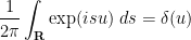
where  is the Dirac delta, we can rewrite this as

which on performing the  integral simplifies to
or after the change of variables  ,
,

We remark that the Kohn-Nirenberg calculus  comes out almost identically, except that the argument
  is replaced with
  . Similarly for the anti-Kohn-Nirenberg calculus (in which is replaced by
  ). The Weyl calculus treats the input variable and the output variable on equal footing, whereas the Kohn-Nirenberg calculus prefers one to the other. In particular, we have the convenient formal identity

so that  formally self-adjoint when is real-valued.
We will take the formula (14) as our definition of the Weyl quantisation  , at least when is a Schwarz function and obeys the weak regularity bounds

for all  , all
, all  , some constant
  , and some constants
  depending on
  . (This is weaker than the symbol bounds that usually arise in the theory of pseudodifferential operators, but will suffice for the discussion here.)
Exercise 1 Show that for and as above, the integrand  is absolutely integrable in , and that the integrand
 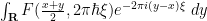 is absolutely integrable in
  , making well-defined. Show in fact that
  is a Schwartz function.
Exercise 2 Show that the above definition agrees with the previous definitions of  and
and  . (One approach is by direct computation; another is to try to make the above formal calculations fully rigorous.)
Exercise 3 (Translation invariance) If obeys the weak regularity bound (16) and  for some
  , show that

where  is the translation operator
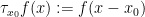
and  is the modulation operator
One can in fact obtain similar symmetries for the entire Weil representation of the (affine) metaplectic group, but we will not do so here.
One can get some intuition as to what the operators do by testing them on gaussian wave packets

It turns out that the Taylor series of around  is a good approximation for the action of on such a packet:
Lemma 1 For any  , one has

as , where  denotes a quantity with
  norm of
  .
.
Thus we have the asymptotic series


with each term of order being of norm . (Note that this does not imply that the series is convergent in , because we have no control of the dependence on of the implied constant in the  notation.)
Proof: (Sketch) By using the symmetries in Exercise 3, we may normalise  . If is a polynomial of degree at most , then the the two sides of (17) agree exactly, with no need for the error term . By subtracting off the order Taylor expansion, we thus see that it suffices to show that

whenever vanishes to order at least at the origin. But this can be verified from (14) and a routine stationary phase computation. 
The same computation allows one to replace the norm by any other of the Frechet norms in the Schwartz space, as long as  are assumed to be of polynomial size in , i.e.
  .
.
From (14), we see that any quantisation is formally an integral operator
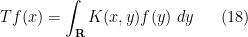
with distributional kernel
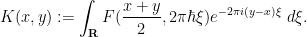
Applying the Fourier inversion formula, we thus see (formally, at least) that any integral operator (18) is also a quantisation where is uniquely determined by the formula

In particular, given two quantisations and  , their composition
  is formally an integral operator with distributional kernel


and hence is formally a quantisation  , where


Thus, for instance,


This integral will, in general, not be absolutely integrable. However, the phase  is only stationary at
  . By using a suitable smooth dyadic decomposition and many integrations by parts, we can then show that this integral can be given a convergent interpretation if obey the weak regularity bound (16). Similarly for other evaluations
  , as well as higher derivatives of
  evaluated at arbitrary points
  . Indeed, with a certain amount of technical effort (which we omit here) we see that is well-defined and obeys (16), and we can rigorously establish the composition law

If and are polynomials, we see (using the fact that any operator has a unique symbol ) that the product given here coincides exactly with the Moyal product (11). As a consequence, by testing on gaussian wave packets using Lemma 1, one can show that this composition law has an asymptotic series given by the Moyal product, thus for any , one has

where the error  obeys the bound (16) (with the constant
  independent of and , and the constant
  depending on but uniform in ). We will not give full details here, but roughly speaking, bound to high order at some point
  , one can subtract off a Taylor polynomial from both and to reduce to the case when at least one of vanishes to high order at , at which point Lemma 1 shows that almost annihilates any gaussian wave packet supported near in phase space, and thus must have very small symbol at
  ; a similar (but more complicated) argument also allows one to control derivatives of the symbol of . In a similar vein, the commutator
 ![{\frac{1}{\hbar} [F(X,D)_W, G(X,D)_W]}](https://s0.wp.com/latex.php?latex=%7B%5Cfrac%7B1%7D%7B%5Chbar%7D+%5BF%28X%2CD%29_W%2C+G%28X%2CD%29_W%5D%7D&bg=ffffff&fg=000000&s=0&c=20201002) of two operators
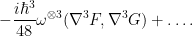
of two operators  with symbols obeying (16) can be described by a symbol with asymptotic series (12); we omit the details. These facts form the basis for the pseudodifferential calculus, which we will not develop further here; see e.g. Taylor’s book or Folland’s book for more details.
We can also relate the Moyal product to the Wigner transform

Comparing this with (19), we see that  can also be interpreted as the symbol of the rank one operator
where  . Given a quantised operator , we (formally, at least) have the relatino

and hence (by (15) and (20)) we see (again formally, at least) that

so that the action of pseudodifferential operators such as can be described through the Wigner transform by some applications of the Moyal product.
Continuing this line of thought, suppose that  is a time-dependent function obeying Schrödinger’s equation

for some real-valued symbol  (representing the Hamiltonian of the system). Passing from the wave function to the density matrix
  , we observe that Schrödinger’s equation implies Heisenberg’s equation
![\displaystyle \partial_t T_\psi = \frac{1}{i\hbar} [H(X,D)_W, T_\psi]](https://s0.wp.com/latex.php?latex=%5Cdisplaystyle++%5Cpartial_t+T_%5Cpsi+%3D+%5Cfrac%7B1%7D%7Bi%5Chbar%7D+%5BH%28X%2CD%29_W%2C+T_%5Cpsi%5D&bg=ffffff&fg=000000&s=0&c=20201002)
and hence (by formal applicaton of the Moyal product)

Applying (12), we see that the Wigner transform of obeys the perturbed Hamiltonian flow equation

This should be compared with the evolution of a classical density function  in phase space with respect to transport along Hamilton’s equation of motion
which is given by the transport equation
Thus we see in the semiclassical limit , the equation of motion for the Wigner transform (21) under the Schrödinger flow converges formally to the equation of motion for a classical density transported under Hamiltonian flow. This is one of the basic manifestations of the correspondence principle relating quantum and classical mechanics, and suggests that the Wigner transform of a wave function is a quantum analogue of a density function in phase space. (But the analogy is not perfect; in particular, the Wigner transform is almost never a non-negative function. See Folland’s book for more discussion.) Making all of these formal calculations and heuristics rigorous is a non-trivial task, requiring the development of the theory of Fourier integral operators, and will not be discussed here.


17 comments
Comments feed for this article
8 October, 2012 at 3:53 am
Fred Lunnon
Section 1 penultimate sentence: F^*(z) definition contradictory?
[Sorry, I don’t see what the problem is here. Note that the use of the asterisk in does not quite denote adjoint or complex conjugation, although it is of course related to those two concepts. -T.]
8 October, 2012 at 5:15 am
David Speyer
I haven’t finished reading to the end yet, but I think the first section would be much easier to read if you started with the observation that Weyl quantization has a symmetry. Namely, let
  be the two dimensional vector space generated by
  and
and  ; let
; let  be the tensor algebra
  and let
  be the ring generated by the operators
  and
and  . If
. If  is in
is in  , and
, and  and
and  are operators from
  , then
 ![[gu, gv]= [u,v]](https://s0.wp.com/latex.php?latex=%5Bgu%2C+gv%5D%3D+%5Bu%2Cv%5D&bg=ffffff&fg=545454&s=0&c=20201002) . So
. So  acts on
  , and the map
  commutes with the
  action.
The Weyl quantization is to lift an element of to the unique preimage in
  which lies in
  . This choice of lifts manifestly respects the
  symmetry.
Therefore, in section 1, there is no need to carry around the and
and  terms. Just use the
  symmetry to reduce to the case where one operator is
  and the other is
  . Moreover, if you want to make life even simpler, you can work with just
  and
and  and restore the powers of
  at the end by homogeneity.
8 October, 2012 at 11:46 am
Terence Tao
Yes, this would work, although for the purposes of Section 1, one could also proceed without the SL_2 invariance just by writing ,
,  and working with A’ and B’ throughout; this does not significantly affect the length of the presentation in this simple case, but is helpful when working with more than two variables as alluded to at the end of Section 1. To me it is a matter of taste – if one wants to prove some identity about finite-dimensional symplectic vector spaces, for instance, does one work in a coordinate free fashion, or does one apply the linear Darboux theorem first to place the symplectic form in a normal form? Both approaches are useful. (Of course, strictly speaking I did not work in a coordinate free fashion in my notes, since I did write everything in terms of A and B, but as mentioned above it is not too difficult to phrase things in the coordinate free formalism.)
8 October, 2012 at 9:47 am
Anonymous
missing expository tag?
8 October, 2012 at 4:52 pm
Steven Stadnicki
Minor typo: your definition of the position operator is missing the factor of
  ; presumably it’s meant to be
  .
.
[Corrected, thanks – T.]
9 October, 2012 at 3:22 am
degosson
Perhaps I missed something, but it seems that you don’t mention a characteristic property of Weyl pseudodifferential operators: they are the only members of the Shubin class that have the property of symplectic/metaplectic covariance (Stein, Wong) . Also, the fact that Weyl operators is the “perfect” quantization procedure in QM is debatable, as has been pointed out by many physicists. In view of Schwartz’s kernel theorem “everything” which is continuous S–>S’ can be written as a Weyl operator, hence any quantum observable could be “dequantized”, but this is physically not true: there are quantum observables which have no classical analogue. A better (i.e. more physical) quantization procedure might very well be the Born-Jordan scheme, which is not always “dequantizable” (see my latest paper “Symplectic covariance properties for Shubin and Born–Jordan pseudo-differential operators” in the Trans. Amer. Math. Soc, online since last Saturday: http://www.ams.org/journals/tran/0000-000-00/).
10 October, 2012 at 5:34 pm
Sam Sachdev
Totally fascinating. Thanks for taking time to make notes on Weyl quantisation.
20 October, 2012 at 3:35 am
����Ԫ
I appreciate it very much that you send every new post of ‘what’s new’, however could you please send me the whole post rather than just a part of it.
Yours sincere,
Han Daoyuan
Sent from my iPad
4 November, 2012 at 6:08 pm
Marcelo de Almeida
Reblogged this on Being simple.
30 November, 2012 at 11:53 am
Lars Hormander « What’s new
[…] to multiplying a phase space distribution by the symbol of that operator, as discussed in this previous blog post. Note that such operators only change the amplitude of the phase space distribution, but not the […]
20 May, 2014 at 11:58 am
Review of wigner nj-Symbols | quantumtetrahedron
[…] Some notes on Weyl quantisation (terrytao.wordpress.com) […]
1 June, 2014 at 8:19 am
Semiclassical Mechanics of the Wigner 6j-Symbol by Aquilanti et al | quantumtetrahedron
[…] Some notes on Weyl quantisation (terrytao.wordpress.com) […]
24 April, 2018 at 1:03 am
João Cortes
Hi professor,
I am trying to understand why the weyl ordering results in an associative product rule for formal series.
I followed your steps up until you combine equations 5,7,9. However, I don’t understand how you “compare coefficients”. In the left hand side of the equation you obtain after that (not numbered), you isolate the term corresponding to the product of the n’th and m’th power of each exponential.
How do you find, in the left hand side, the terms that correspond to this?
Thanks
24 April, 2018 at 7:00 am
Terence Tao
Collect the terms whose total degree is
  and whose
  total degree is
  .
.
27 April, 2018 at 4:21 am
João Cortes
thanks for your reply. It’s weird being able to communicate with you. The wonders of the internet! and m $B’s$) correspond to different polynomials, using the Weyl prescription?
I have another question, if you don’t mind.
Do you know any simple argument to show that different orders of a monomial of operators (that is, different ways of multiplying n
27 April, 2018 at 2:23 pm
Terence Tao
Look at what such a monomial does to a monomial .
.
19 May, 2023 at 7:17 am
alwill
Thanks for the derivation, this helps me for doing my homework.