The wave equation is usually expressed in the form

where  is a function of both time
  and space
  , with
  being the Laplacian operator. One can generalise this equation in a number of ways, for instance by replacing the spatial domain
  with some other manifold and replacing the Laplacian with the Laplace-Beltrami operator or adding lower order terms (such as a potential, or a coupling with a magnetic field). But for sake of discussion let us work with the classical wave equation on . We will work formally in this post, being unconcerned with issues of convergence, justifying interchange of integrals, derivatives, or limits, etc.. One then has a conserved energy
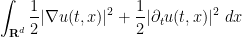
which we can rewrite using integration by parts and the  inner product
  on as
on as

A key feature of the wave equation is finite speed of propagation: if, at time  (say), the initial position
  and initial velocity
  are both supported in a ball
  , then at any later time
  , the position
  and velocity
  are supported in the larger ball
  . This can be seen for instance (formally, at least) by inspecting the exterior energy

and observing (after some integration by parts and differentiation under the integral sign) that it is non-increasing in time, non-negative, and vanishing at time .
The wave equation is second order in time, but one can turn it into a first order system by working with the pair  rather than just the single field , where
  is the velocity field. The system is then


and the conserved energy is now

Finite speed of propagation then tells us that if  are both supported on
  , then
  are supported on for all . One also has time reversal symmetry: if
  is a solution, then
  is a solution also, thus for instance one can establish an analogue of finite speed of propagation for negative times
  using this symmetry.
If one has an eigenfunction

of the Laplacian, then we have the explicit solutions


of the wave equation, which formally can be used to construct all other solutions via the principle of superposition.
When one has vanishing initial velocity  , the solution is given via functional calculus by
and the propagator  can be expressed as the average of half-wave operators:

One can view  as a minor of the full wave propagator

which is unitary with respect to the energy form (1), and is the fundamental solution to the wave equation in the sense that

Viewing the contraction  as a minor of a unitary operator is an instance of the “dilation trick“.
It turns out (as I learned from Yuval Peres) that there is a useful discrete analogue of the wave equation (and of all of the above facts), in which the time variable  now lives on the integers
  rather than on
  , and the spatial domain can be replaced by discrete domains also (such as graphs). Formally, the system is now of the form


where is now an integer,  take values in some Hilbert space (e.g.
  functions on a graph
  ), and
  is some operator on that Hilbert space (which in applications will usually be a self-adjoint contraction). To connect this with the classical wave equation, let us first consider a rescaling of this system

where  is a small parameter (representing the discretised time step), now takes values in the integer multiples
  of
of  , and
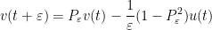
, and  is the wave propagator operator
  or the heat propagator
  (the two operators are different, but agree to fourth order in ). One can then formally verify that the wave equation emerges from this rescaled system in the limit
  . (Thus, is not exactly the direct analogue of the Laplacian , but can be viewed as something like
 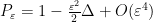 in the case of small , or
  if we are not rescaling to the small case. The operator is sometimes known as the diffusion operator)
Assuming is self-adjoint, solutions to the system (3) formally conserve the energy

This energy is positive semi-definite if is a contraction. We have the same time reversal symmetry as before: if solves the system (3), then so does . If one has an eigenfunction

to the operator , then one has an explicit solution

to (3), and (in principle at least) this generates all other solutions via the principle of superposition.
Finite speed of propagation is a lot easier in the discrete setting, though one has to offset the support of the “velocity” field  by one unit. Suppose we know that has unit speed in the sense that whenever
  is supported in a ball
  , then
  is supported in the ball
  . Then an easy induction shows that if
  are supported in
  respectively, then are supported in
  .
.
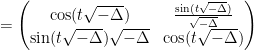
The fundamental solution  to the discretised wave equation (3), in the sense of (2), is given by the formula

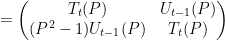
where  and
and  are the Chebyshev polynomials of the first and second kind, thus

and

In particular, is now a minor of  , and can also be viewed as an average of
  with its inverse
  :
:

As before, is unitary with respect to the energy form (4), so this is another instance of the dilation trick in action. The powers  and
and  are discrete analogues of the heat propagators
  and wave propagators
  respectively.
One nice application of all this formalism, which I learned from Yuval Peres, is the Varopoulos-Carne inequality:
Theorem 1 (Varopoulos-Carne inequality) Let be a (possibly infinite) regular graph, let  , and let
  be vertices in . Then the probability that the simple random walk at
  lands at
  at time
  is at most
  , where
  is the graph distance.
This general inequality is quite sharp, as one can see using the standard Cayley graph on the integers . Very roughly speaking, it asserts that on a regular graph of reasonably controlled growth (e.g. polynomial growth), random walks of length concentrate on the ball of radius  or so centred at the origin of the random walk.
Proof: Let  be the graph Laplacian, thus

for any  , where
  is the degree of the regular graph and sum is over the vertices that are adjacent to . This is a contraction of unit speed, and the probability that the random walk at lands at at time is

where  are the Dirac deltas at
  . Using (5), we can rewrite this as

where we are now using the energy form (4). We can write

where  is the simple random walk of length on the integers, that is to say
  where
where  are independent uniform Bernoulli signs. Thus we wish to show that

By finite speed of propagation, the inner product here vanishes if  . For
. For  we can use Cauchy-Schwarz and the unitary nature of to bound the inner product by
  . Thus the left-hand side may be upper bounded by
and the claim now follows from the Chernoff inequality. 
This inequality has many applications, particularly with regards to relating the entropy, mixing time, and concentration of random walks with volume growth of balls; see this text of Lyons and Peres for some examples.
For sake of comparison, here is a continuous counterpart to the Varopoulos-Carne inequality:
Theorem 2 (Continuous Varopoulos-Carne inequality) Let  , and let
  be supported on compact sets
  respectively. Then

where  is the Euclidean distance between
  and .
and .
Proof: By Fourier inversion one has
for any real  , and thus

By finite speed of propagation, the inner product  vanishes when
  ; otherwise, we can use Cauchy-Schwarz and the contractive nature of
  to bound this inner product by
  . Thus

Bounding  by
by  , we obtain the claim.
Observe that the argument is quite general and can be applied for instance to other Riemannian manifolds than .


21 comments
Comments feed for this article
5 November, 2014 at 7:18 pm
Nick Cook
In the last line, the L^2 norms should be of f,g rather than F,G.
[Corrected, thanks – T.]
5 November, 2014 at 7:51 pm
Nick Cook
Also, shouldn’t we use the bound ? This leads to another
  in the reciprocal for the bound in the theorem.
[Corrected, thanks – T.]
6 November, 2014 at 6:44 am
Anonymous
\colon instead of : for maps.
[Corrected, thanks – T.]
7 November, 2014 at 2:55 am
Anonymous
Terry: Have you really corrected it? :)
[Web version is now corrected also. -T.]
6 November, 2014 at 7:01 am
observer
Probabilistic ideas can also be used to get other generalized laplacians, e.g., (18) in http://www.stt.msu.edu/~mcubed/Relativistic.pdf.
6 February, 2015 at 10:57 pm
Aza
Relativistic laplacian?
6 November, 2014 at 7:11 am
Pedro Lauridsen Ribeiro
There is a whole family of “finite speed propagation” estimates for spin systems with local interactions, called Lieb-Robinson bounds (http://en.wikipedia.org/wiki/Lieb-Robinson_bounds), which look quite similar to the (discrete) Varopoulos-Carne inequality. It would be interesting to know if there is a deeper relation between both. (by the way, it is spelled “Varopoulos” and not “Varopoulous”)
[Corrected, thanks – T.]
6 November, 2014 at 8:00 pm
luca
The operator P defined at the beginning of the proof of Theorem 1 is the random walk (or “diffusion”) operator; the Laplacian of the graph is I-P.
[Some comments added on this – T.]
7 November, 2014 at 6:33 am
timur
Does there exist similar discretized framework for nonlinear equations, such as Yang-Mills or wave maps?
7 November, 2014 at 9:02 am
Terence Tao
I don’t know about these specific equations. Several of the standard completely integrable systems (e.g. KdV, cubic 1D NLS) have discrete models (some in which space is discretised, and some in which both space and time are discretised, i.e. lattice models); see e.g. the literature on lattice KdV equations.
Presumably the discrete wave equation discussed here has a Lagrangian formulation, in which case it looks plausible that one could then derive a discrete Yang-Mills or wave maps equation by modifying the Lagrangian in the obvious ways. I might try to play with finding such a formulation later, though I won’t have much time for this in the next few days.
9 November, 2014 at 3:15 pm
Terence Tao
For what it’s worth, I did compute that solutions to the discretised wave equation are critical points for the Lagrangian
but it is not obvious to me how to adapt this Lagrangian to a wave map or Yang-Mills setting.
8 November, 2014 at 2:57 am
M
thank you
8 November, 2014 at 3:39 pm
Marcelo de Almeida
Reblogged this on Being simple.
9 November, 2014 at 3:08 pm
notedscholar
There are quite a few symbols here. Perhaps I’ll reblog it.
9 November, 2014 at 3:09 pm
notedscholar
Reblogged this on Science and Math Defeated and commented:
Can anyone please explain this to me? I can’t really figure out what the symbols mean.
10 November, 2014 at 5:38 pm
notedscholar
Who on earth besides me is rating my comments down?
12 November, 2014 at 6:17 am
Anonymous
Me!
12 November, 2014 at 5:24 am
MrCactu5 (@MonsieurCactus)
Did you really take cosine of the Laplacian, ? I am always confused because you can talk about diffusion and you can talk about waves.
12 November, 2014 at 6:02 am
MrCactu5 (@MonsieurCactus)
I am not so sure. If your two points are very close VC inequality says the probability tends to zero. Even if G is finite?
The content of the Varopolos-Carne inequality is a bound that works for any Cayley graph?
The VC inequality in the case of the Integers can be proven using the DeMoivre-Laplace limit theorem. Or using the the entropy formula.
19 November, 2014 at 12:34 pm
Anon
The solutions to the discretized wave equation can be used to cluster graphs…..
7 December, 2015 at 12:17 pm
Diegus
got it until time discretization eq (3) as {\varepsilon} > 0 as P not for “heat propagation” but as a -discretization unit- where U(t) = U_t for zeroing epsilon where U(1) = U only if epsilon closes in to zero.. the opposite if U(1) for stateless epsilon?