I recently learned about a curious operation on square matrices known as sweeping, which is used in numerical linear algebra (particularly in applications to statistics), as a useful and more robust variant of the usual Gaussian elimination operations seen in undergraduate linear algebra courses. Given an  matrix
  (with, say, complex entries) and an index
  , with the entry
  non-zero, the sweep
 ![{\hbox{Sweep}_k[A] = (\hat a_{ij})_{1 \leq i,j \leq n}}](https://s0.wp.com/latex.php?latex=%7B%5Chbox%7BSweep%7D_k%5BA%5D+%3D+%28%5Chat+a_%7Bij%7D%29_%7B1+%5Cleq+i%2Cj+%5Cleq+n%7D%7D&bg=ffffff&fg=000000&s=0&c=20201002) of
of  at
at  is the matrix given by the formulae
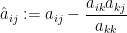


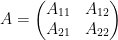
for all 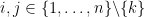 . Thus for instance if
  , and is written in block form as

for some  row vector
  ,
,  column vector
  , and
, and  minor
minor  , one has
![\displaystyle \hbox{Sweep}_1[A] = \begin{pmatrix} -1/a_{11} & X / a_{11} \\ Y/a_{11} & B - a_{11}^{-1} YX \end{pmatrix}. \ \ \ \ \ (2)](https://s0.wp.com/latex.php?latex=%5Cdisplaystyle++%5Chbox%7BSweep%7D_1%5BA%5D+%3D+%5Cbegin%7Bpmatrix%7D+-1%2Fa_%7B11%7D+%26+X+%2F+a_%7B11%7D+%5C%5C+Y%2Fa_%7B11%7D+%26+B+-+a_%7B11%7D%5E%7B-1%7D+YX+%5Cend%7Bpmatrix%7D.+%5C+%5C+%5C+%5C+%5C+%282%29&bg=ffffff&fg=000000&s=0&c=20201002)
The inverse sweep operation ![{\hbox{Sweep}_k^{-1}[A] = (\check a_{ij})_{1 \leq i,j \leq n}}](https://s0.wp.com/latex.php?latex=%7B%5Chbox%7BSweep%7D_k%5E%7B-1%7D%5BA%5D+%3D+%28%5Ccheck+a_%7Bij%7D%29_%7B1+%5Cleq+i%2Cj+%5Cleq+n%7D%7D&bg=ffffff&fg=000000&s=0&c=20201002) is given by a nearly identical set of formulae:
is given by a nearly identical set of formulae:


for all . One can check that these operations invert each other. Actually, each sweep turns out to have order  , so that
  : an inverse sweep performs the same operation as three forward sweeps. Sweeps also preserve the space of symmetric matrices (allowing one to cut down computational run time in that case by a factor of two), and behave well with respect to principal minors; a sweep of a principal minor is a principal minor of a sweep, after adjusting indices appropriately.
Remarkably, the sweep operators all commute with each other:  . If and we perform the first sweeps (in any order) to a matrix
with  a
a  minor,
  a
a  matrix, a
  matrix, and
  a
a  matrix, one obtains the new matrix
![\displaystyle \hbox{Sweep}_1 \dots \hbox{Sweep}_k[A] = \begin{pmatrix} -A_{11}^{-1} & A_{11}^{-1} A_{12} \\ A_{21} A_{11}^{-1} & A_{22} - A_{21} A_{11}^{-1} A_{12} \end{pmatrix}.](https://s0.wp.com/latex.php?latex=%5Cdisplaystyle++%5Chbox%7BSweep%7D_1+%5Cdots+%5Chbox%7BSweep%7D_k%5BA%5D+%3D+%5Cbegin%7Bpmatrix%7D+-A_%7B11%7D%5E%7B-1%7D+%26+A_%7B11%7D%5E%7B-1%7D+A_%7B12%7D+%5C%5C+A_%7B21%7D+A_%7B11%7D%5E%7B-1%7D+%26+A_%7B22%7D+-+A_%7B21%7D+A_%7B11%7D%5E%7B-1%7D+A_%7B12%7D+%5Cend%7Bpmatrix%7D.&bg=ffffff&fg=000000&s=0&c=20201002)
Note the appearance of the Schur complement in the bottom right block. Thus, for instance, one can essentially invert a matrix by performing all  sweeps:
![\displaystyle \hbox{Sweep}_1 \dots \hbox{Sweep}_n[A] = -A^{-1}.](https://s0.wp.com/latex.php?latex=%5Cdisplaystyle++%5Chbox%7BSweep%7D_1+%5Cdots+%5Chbox%7BSweep%7D_n%5BA%5D+%3D+-A%5E%7B-1%7D.&bg=ffffff&fg=000000&s=0&c=20201002)
If a matrix has the form

for a minor , column vector , row vector , and scalar  , then performing the first
  sweeps gives
![\displaystyle \hbox{Sweep}_1 \dots \hbox{Sweep}_{n-1}[A] = \begin{pmatrix} -B^{-1} & B^{-1} X \\ Y B^{-1} & a - Y B^{-1} X \end{pmatrix}](https://s0.wp.com/latex.php?latex=%5Cdisplaystyle++%5Chbox%7BSweep%7D_1+%5Cdots+%5Chbox%7BSweep%7D_%7Bn-1%7D%5BA%5D+%3D+%5Cbegin%7Bpmatrix%7D+-B%5E%7B-1%7D+%26+B%5E%7B-1%7D+X+%5C%5C+Y+B%5E%7B-1%7D+%26+a+-+Y+B%5E%7B-1%7D+X+%5Cend%7Bpmatrix%7D+&bg=ffffff&fg=000000&s=0&c=20201002)
and all the components of this matrix are usable for various numerical linear algebra applications in statistics (e.g. in least squares regression). Given that sweeps behave well with inverses, it is perhaps not surprising that sweeps also behave well under determinants: the determinant of can be factored as the product of the entry and the determinant of the matrix formed from ![{\hbox{Sweep}_k[A]}](https://s0.wp.com/latex.php?latex=%7B%5Chbox%7BSweep%7D_k%5BA%5D%7D&bg=ffffff&fg=000000&s=0&c=20201002) by removing the
by removing the  row and column. As a consequence, one can compute the determinant of fairly efficiently (so long as the sweep operations don’t come close to dividing by zero) by sweeping the matrix for
  in turn, and multiplying together the
  entry of the matrix just before the sweep for to obtain the determinant.
It turns out that there is a simple geometric explanation for these seemingly magical properties of the sweep operation. Any matrix creates a graph ![{\hbox{Graph}[A] := \{ (X, AX): X \in {\bf R}^n \}}](https://s0.wp.com/latex.php?latex=%7B%5Chbox%7BGraph%7D%5BA%5D+%3A%3D+%5C%7B+%28X%2C+AX%29%3A+X+%5Cin+%7B%5Cbf+R%7D%5En+%5C%7D%7D&bg=ffffff&fg=000000&s=0&c=20201002) (where we think of
(where we think of  as the space of column vectors). This graph is an -dimensional subspace of
  . Conversely, most subspaces of arises as graphs; there are some that fail the vertical line test, but these are a positive codimension set of counterexamples.
We use  to denote the standard basis of , with
  the standard basis for the first factor of and
  the standard basis for the second factor. The operation of sweeping the entry then corresponds to a ninety degree rotation
  in the
  plane, that sends
  to
to  (and to
  ), keeping all other basis vectors fixed: thus we have
![\displaystyle \hbox{Graph}[ \hbox{Sweep}_k[A] ] = \hbox{Rot}_k \hbox{Graph}[A]](https://s0.wp.com/latex.php?latex=%5Cdisplaystyle++%5Chbox%7BGraph%7D%5B+%5Chbox%7BSweep%7D_k%5BA%5D+%5D+%3D+%5Chbox%7BRot%7D_k+%5Chbox%7BGraph%7D%5BA%5D+&bg=ffffff&fg=000000&s=0&c=20201002)
for generic (more precisely, those with non-vanishing entry ). For instance, if and is of the form (1), then ![{\hbox{Graph}[A]}](https://s0.wp.com/latex.php?latex=%7B%5Chbox%7BGraph%7D%5BA%5D%7D&bg=ffffff&fg=000000&s=0&c=20201002) is the set of tuples
is the set of tuples  obeying the equations


The image of  under
under  is
is  . Since we can write the above system of equations (for
  ) as
) as
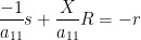
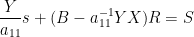
we see from (2) that ![{\hbox{Rot}_1 \hbox{Graph}[A]}](https://s0.wp.com/latex.php?latex=%7B%5Chbox%7BRot%7D_1+%5Chbox%7BGraph%7D%5BA%5D%7D&bg=ffffff&fg=000000&s=0&c=20201002) is the graph of
is the graph of ![{\hbox{Sweep}_1[A]}](https://s0.wp.com/latex.php?latex=%7B%5Chbox%7BSweep%7D_1%5BA%5D%7D&bg=ffffff&fg=000000&s=0&c=20201002) . Thus the sweep operation is a multidimensional generalisation of the high school geometry fact that the line
. Thus the sweep operation is a multidimensional generalisation of the high school geometry fact that the line  in the plane becomes
  after applying a ninety degree rotation.
It is then an instructive exercise to use this geometric interpretation of the sweep operator to recover all the remarkable properties about these operations listed above. It is also useful to compare the geometric interpretation of sweeping as rotation of the graph to that of Gaussian elimination, which instead shears and reflects the graph by various elementary transformations (this is what is going on geometrically when one performs Gaussian elimination on an augmented matrix). Rotations are less distorting than shears, so one can see geometrically why sweeping can produce fewer numerical artefacts than Gaussian elimination.


26 comments
Comments feed for this article
7 October, 2015 at 11:44 am
grpaseman
Interesting! This reminds me of an analogous operation for when a_{11} is 0: multiply the first row by -1, add it to all the other rows, and then multiply the changed columns by -1. For arbitrary matrices this looks like a mess, but I was working with 0-1 matrices and wanted to preserve absolute value of the determinant. I might consider looking at those matrices again from a geometric viewpoint. Thanks for the post.
7 October, 2015 at 11:51 am
Anonymous
may want to add an “expository” tag
[Added, thanks – T.]
7 October, 2015 at 2:38 pm
A
YX in (2) instead of XY.
[Corrected, thanks – T.]
7 October, 2015 at 3:49 pm
Anonymous
This seems to be Gauss-Jordan elimination written with 1 table rather than 2 where you re-use the columns of the first table to hold the emerging columns of the 2nd table? That is you eliminate both below and above the main diagonal before you proceed to the next column. Because of this you can re-use the columns of A (or U) to hold the columns of A^{-1}. This also explains why the sweeps commute (zeros in the right place of the columns you have already eliminated).
In LU factorization terms you are interleaving the elementary factors of L^{-1} with that of U^{-1}. Not sure if my verbal description makes sense to anyone….
In any case this does not seem to be a good idea numerically without incorporating some form of pivoting.
7 October, 2015 at 10:09 pm
Dr. Seppo
Sweep seems to be the same as gyration, aside from a sign change. Gyrations have been studied or used in linear programming where dependent and independent variables are swapped, Tucker has been mentioned in that context. The sign change is clever though as it preserves symmetry, so the “new name” sweep is perhaps justified — but you can find old references with the search term “gyration”.
8 October, 2015 at 1:04 am
kante
The sweep operation is also known as Principal Pivot Transform, (as far as I know) introduced by Tucker [A Combinatorial Equivalence of Matrices. In R. Bellman and M. Hall Jr editors, Combinatorial Analysis, pages 129–140. AMS, Providence, 1960] (see the survey by Tsatsomeros [M.J. Tsatsomeros. Principal Pivot Transforms: Properties and Applications. Linear Algebra and its Applications 307(1-3):151–165, 2000]). It is funny because it is related to minors in (Delta-)matroids (and so Graph Minor), see for instance [S. Oum. Rank-Width and Well-Quasi-Ordering of Skew-Symmetric or
Symmetric Matrices. Linear Algebra and its Applications 436(7):2008–2036, 2012.]
8 October, 2015 at 3:51 am
tomcircle
Reblogged this on Math Online Tom Circle and commented:
Interesting!
8 October, 2015 at 4:58 am
MatjazG
Very interesting! Didn’t encounter it before but it just so happens that your post comes at a good time, since I think it could be useful for my work. :)
I have a question, though: would an obvious generalization to a “fractional sweep”:![\hbox{Sweep}_k^\alpha[A] = A \cos \alpha + \hbox{Sweep}_k[A] \sin \alpha](https://s0.wp.com/latex.php?latex=%5Chbox%7BSweep%7D_k%5E%5Calpha%5BA%5D+%3D+A+%5Ccos+%5Calpha+%2B+%5Chbox%7BSweep%7D_k%5BA%5D+%5Csin+%5Calpha&bg=ffffff&fg=545454&s=0&c=20201002) be a useful concept? Geometrically it would correspond to a rotation by an angle
be a useful concept? Geometrically it would correspond to a rotation by an angle  in the
  plane and hence algebraically to a fractional power
  of the unitary (under the canonical scalar product on
  from your post) operator
  .
.
[I ask because for example the other fractional transforms many times turn out to be quite useful. For example, the fractional Fourier transform, which is just a rotation by the angle of the Wigner quasiprobability function (if I remember correctly) is useful in many areas and also turns out to be the evolution operator for a particle in a linear harmonic oscillator potential in quantum mechanics, where
  changes linearly with time.]
Fractional sweeps would still be commutative and should thus, for example, give a simple algorithmic way to calculate the fractional power
  of a
of a  matrix
  when applied in succession for all
  with the same
  :
:
if my thinking is correct:
If is rational then
 ![(\hbox{Sweep}_1^\alpha \dots \hbox{Sweep}_n^\alpha)^q[A] = (\hbox{Sweep}_1 \dots \hbox{Sweep}_n)^p[A] = (-A^{-1})^p = (-1)^p A^{-p}](https://s0.wp.com/latex.php?latex=%28%5Chbox%7BSweep%7D_1%5E%5Calpha+%5Cdots+%5Chbox%7BSweep%7D_n%5E%5Calpha%29%5Eq%5BA%5D+%3D+%28%5Chbox%7BSweep%7D_1+%5Cdots+%5Chbox%7BSweep%7D_n%29%5Ep%5BA%5D+%3D+%28-A%5E%7B-1%7D%29%5Ep+%3D+%28-1%29%5Ep+A%5E%7B-p%7D&bg=ffffff&fg=545454&s=0&c=20201002) , and thus:
, and thus: ![\hbox{Sweep}_1^\alpha \dots \hbox{Sweep}_n^\alpha[A] = (-1)^\frac{p}{q} A^{-\frac{p}{q}} = (-1)^\alpha A^{-\alpha}](https://s0.wp.com/latex.php?latex=%5Chbox%7BSweep%7D_1%5E%5Calpha+%5Cdots+%5Chbox%7BSweep%7D_n%5E%5Calpha%5BA%5D+%3D+%28-1%29%5E%5Cfrac%7Bp%7D%7Bq%7D+A%5E%7B-%5Cfrac%7Bp%7D%7Bq%7D%7D+%3D+%28-1%29%5E%5Calpha+A%5E%7B-%5Calpha%7D&bg=ffffff&fg=545454&s=0&c=20201002) . Since this is a continuous operation in
. Since this is a continuous operation in  and rational numbers are dense in the reals the same relation should hold for all
  . (Perhaps not completely rigorous, I guess, but I think it should hold.)
And I’m sure there are other examples where fractional sweeps could be useful.
P.S. I’m a physicist, not a mathematician, but I’ve been reading your blog for the past two years and it inspires me to learn more things from pure mathematics and also continually gives me fresh ideas for problem solving when dealing with my physical models.
P.P.S. Also, congratulations on solving the Erdos discrepancy problem! :)
8 October, 2015 at 11:36 am
Terence Tao
It seems is a bit more complicated than this; rotation acts linearly on a graph, but not on the function defining the graph. One can see this even in one dimension: a line
  rotated by
  becomes a line with slope
  (tangent addition rule). The corresponding formula in higher dimensions should be computable but looks a bit messy.
8 October, 2015 at 11:43 am
Avi Levy
Does the formula become simpler if we identify the graph with
with  , pairing up the real coordinates to produce complex coordinates and think in terms of complex multiplication?
8 October, 2015 at 12:59 pm
MatjazG
Thank you your the reply! :) Ah, yes, I see the mistake. I was a bit hasty there; should’ve been more careful … I will try (<- emphasis) to compute the correct formula anyway, as an exercise. :p
8 October, 2015 at 2:30 pm
MatjazG
Not that hard after all, but I see I made another mistake above: to have the notation that![\hbox{Sweep}_k^1[A] = \hbox{Sweep}_k[A]](https://s0.wp.com/latex.php?latex=%5Chbox%7BSweep%7D_k%5E1%5BA%5D+%3D+%5Chbox%7BSweep%7D_k%5BA%5D&bg=ffffff&fg=545454&s=0&c=20201002) a fractional sweep meant as the power
a fractional sweep meant as the power  of
of  corresponds to a rotation by
  (not
(not  ) of the graph in the
  plane.
A rotation of the matrix graph![\hbox{Graph}[A]](https://s0.wp.com/latex.php?latex=%5Chbox%7BGraph%7D%5BA%5D&bg=ffffff&fg=545454&s=0&c=20201002) by
by  in the
  plane means that we send
  to
to  , where:
So we want to express the original equations:
as equations for in terms of
  .
.
We can do this easily by first: in terms of
  (of course, the equations look the same as for the other way around, just with
  instead of
  ),
), from
from  by from the first original equation, and finally,
 into the second original equation.
– using the orthogonality of rotations to express
– substituting that into both original equations,
– expressing
– putting the expression for
We get:
where:
which together form the matrix![\hbox{Sweep}_1^\alpha[A]](https://s0.wp.com/latex.php?latex=%5Chbox%7BSweep%7D_1%5E%5Calpha%5BA%5D&bg=ffffff&fg=545454&s=0&c=20201002) (where
(where  ).
).
Explicitly:
and analogously for for other
  (just switch the order of the basis or apply permutation matrices around this). :)
Here are
are  matrices,
  are
are  matrices,
  are
are  row vectors
  are $n – 1 \times 1$ column vectors and
  are scalars.
Let’s do a sanity check: verifying the limit we get the expected identity transformation
 ![A' = \hbox{Sweep}^0_1[A] = A](https://s0.wp.com/latex.php?latex=A%27+%3D+%5Chbox%7BSweep%7D%5E0_1%5BA%5D+%3D+A&bg=ffffff&fg=545454&s=0&c=20201002) and verifying the limit
and verifying the limit  (
( ) we get the normal sweep
 ![A' = \hbox{Sweep}^1_1[A] = \hbox{Sweep}_1[A]](https://s0.wp.com/latex.php?latex=A%27+%3D+%5Chbox%7BSweep%7D%5E1_1%5BA%5D+%3D+%5Chbox%7BSweep%7D_1%5BA%5D&bg=ffffff&fg=545454&s=0&c=20201002) .
.
The condition (unless
  ), also passes the sanity check for
  (no restriction on
  ) and
) and  (the condition
  ), of course. :)
Of course, only works when
  , since otherwise we get zero denominators, necessarily giving an undefined (at least)
  (unless
  ).
).
The equations for a fractional sweep might look a bit messy, but still not that much. They are basically almost as easy to implement on a computer as those for regular sweeps, and for many consecutive sweeps with the same
  you basically need only a few more additions and multiplications per sweep to get the end result, since you can pre-compute
  and
and  only once, at the beginning of the computation.
For example, if you want to compute a fractional power of a matrix as
as ![A^\alpha = \hbox{Sweep}_1^{-\alpha} \dots \hbox{Sweep}_n^{-\alpha}[-A]](https://s0.wp.com/latex.php?latex=A%5E%5Calpha+%3D+%5Chbox%7BSweep%7D_1%5E%7B-%5Calpha%7D+%5Cdots+%5Chbox%7BSweep%7D_n%5E%7B-%5Calpha%7D%5B-A%5D&bg=ffffff&fg=545454&s=0&c=20201002) , as mentioned in my previous post, you can use this algorithm as an in-place computation, without the need for e.g. an eigenvalue decomposition. (My first guess to compute
, as mentioned in my previous post, you can use this algorithm as an in-place computation, without the need for e.g. an eigenvalue decomposition. (My first guess to compute  would be to compute the eigenvalues, put them to some power and then recompose the matrix; with fractional sweeps this is unnecessary – but perhaps there is an even better way?)
I hope someone finds this useful. Anyway, it was nice thinking about this. :) I just hope I haven’t made any more mistakes … :p
P.S. after
after ![\hbox{Sweep}_1[A]](https://s0.wp.com/latex.php?latex=%5Chbox%7BSweep%7D_1%5BA%5D&bg=ffffff&fg=545454&s=0&c=20201002) ) there is an
) there is an  term (which is scalar), which should instead by
  (matrix/tensor).
While writing this I noticed a mistake in your original blog post: in the last equation that has its own line (expressing
[Corrected, thanks – T.]
8 October, 2015 at 11:06 pm
MatjazG
P.S. Never mind about calculating by fractional sweeps. Fractional sweeps (of course) don’t produce that as a result. :(
P.P.S. I’m also sorry for spamming the comments so much in the last day.
8 October, 2015 at 11:38 pm
Anonymous
Which values have the above commutative property (independent of the matrix graph!) for all their corresponding sweep operators?
 values can be larger for certain symmetries of the matrix graph.
It seems that this (smallest) set of
9 October, 2015 at 4:40 am
MatjazG
Commutativity should hold for all and all
  in the sense that
  .
.
This is because the only thing that does is that it rotates the graph of an arbitrary matrix in the
  plane by an angle
  , leaving the rest of the matrix graph (i.e. all other planes
  for
for  ) completely unchanged.
So we have two cases to check: either and we have proven commutativity by the fact that they operate on different planes independently, or
  and then commutativity holds since rotations in a single plane are always commutative (i.e. the group
  is commutative).
P.S. in here, restoring a bit of symmetry and simplicity:
If I am posting yet another comment, let me just throw these more elegant (but equivalent) expressions for the fractional sweep
where .
.
Let me also add that I’ve checked these formulas, so that when you applying a fractional sweep first with and then do another one with
  after it, that the result is indeed the same as doing a single fractional sweep with
  (I checked the general case with Mathematica and separately by hand for general
  and also for
  ). In other words, I did the sanity check that:
  latex \hbox{Sweep}_1^\beta = \hbox{Sweep}_1^{\alpha+\beta}$, which also proves commutativity when
  .
.
So the above expressions for a fractional sweep should really be correct now! :)
P.P.S.
A note about commutativity:
We could always conceive of more contrived generalized operations which do not commute, like for example a “fractional multi-sweep”:![\hbox{Sweep}_k^\alpha[F]](https://s0.wp.com/latex.php?latex=%5Chbox%7BSweep%7D_k%5E%5Calpha%5BF%5D&bg=ffffff&fg=545454&s=0&c=20201002) , where
, where  is now a multi-linear map with
  input vectors from
  and one output vector in
  , and where
  is a vector with
  components. A fractional mult-sweep would act on the graph
 ![{\hbox{Graph}[F] := \{ (X_1, \dots, X_m, F(X_1, \dots, X_m)): X_1, \dots X_m \in {\bf R}^n \}} \subset {\bf R}^{(m+1)n}](https://s0.wp.com/latex.php?latex=%7B%5Chbox%7BGraph%7D%5BF%5D+%3A%3D+%5C%7B+%28X_1%2C+%5Cdots%2C+X_m%2C+F%28X_1%2C+%5Cdots%2C+X_m%29%29%3A+X_1%2C+%5Cdots+X_m+%5Cin+%7B%5Cbf+R%7D%5En+%5C%7D%7D+%5Csubset+%7B%5Cbf+R%7D%5E%7B%28m%2B1%29n%7D&bg=ffffff&fg=545454&s=0&c=20201002) of the multi-linear map
of the multi-linear map  , with canonical basis vectors
  , by rotating it in the
  subspace with a rotation from the group
  described by the vector
  . (The vector
  has the same number components as there are independent generators of
  so we have precisely the correct number of degrees of freedom to describe rotations in the the
  dimensional subspace spanned by
  .) The regular fractional sweep is just the special case when
  .
.
Now, fractional multi-sweeps also commute when (i.e. it still holds that
  in that case) since subspaces for different
  are independent, but when
  they in general do not commute any more for arbitrary
  , since the group
  is non-abelian for
  . Whether or not “fractional multi-sweeps” would be useful for anything though, I have no idea (I don’t know that even about regular fractional sweeps now :p).
P.P.P.S. is a rotation by an angle
  in the time-frequency domain).
Generalizing further in another direction: the fractional Fourier transformation is a special case of a linear canonical transformation (LCT; also known as the Collins diffraction integral when used to describe light beam propagation through linear elements in paraxial optics) which is a general linear transformation in the time-frequency domain of a function (for example, a fractional Fourier transform with the fraction
Analogously, would it then be interesting to consider what happens to the matrix when we apply a more general linear transformation to its graph
 ![\hbox{Graph}[A]](https://s0.wp.com/latex.php?latex=%5Chbox%7BGraph%7D%5BA%5D&bg=ffffff&fg=545454&s=0&c=20201002) (either restricted to a
(either restricted to a  plane or not)?
Anyway, you can always generalize almost anything, but it would be good if it could be used for something non-trivial at some point … :p
9 October, 2015 at 8:18 am
MatjazG
I just can’t seem to leave this topic alone, it just fascinates me too much. :p What I’m worried about, though, is if I am derailing the discussion under this post too much. Would it be better to move/post all of this somewhere else instead, so it doesn’t take up so much space on this blog? If that would be better, I will write these things down somewhere else; I just feel the urge to write down my findings somewhere … :p Also, any input is greatly appreciated.
—
So, I have obtained the general formula for what happens to an matrix
  when we apply a linear transformation on its graph
 ![\hbox{Graph}[A]](https://s0.wp.com/latex.php?latex=%5Chbox%7BGraph%7D%5BA%5D&bg=ffffff&fg=545454&s=0&c=20201002) in the
in the  plane, leaving the rest of the graph unmodified. Specifically, lets take
  and express the coordinates
  after a linear transformation transformation
  in the
  plane as:
where is a
is a  matrix,
  are scalars and
  are
are  column vectors.
Then we want the following:
where , to be equivalent to:
where is the matrix corresponding to the transformed graph. Here,
  are scalars,
  are
are  row vectors,
  are
are  column vectors,
  are
are  matrices and
  are
are  matrices. The formulas I are obtained for
  are the following:
where and
and  is the determinant of the matrix
  . This works when:
  (the matrix
  should probably also be non-degenerate = invertible = with
  ).
).
This neatly generalizes the fractional sweep, which is just a special case when: , the special case of which is the regular (full) sweep with:
  , i.e.
  in the fractional sweep.
For convenience, let’s define the above obtained![A' = \hbox{Sweep}^M_1[A]](https://s0.wp.com/latex.php?latex=A%27+%3D+%5Chbox%7BSweep%7D%5EM_1%5BA%5D&bg=ffffff&fg=545454&s=0&c=20201002) as the “general linear sweep” of the matrix
as the “general linear sweep” of the matrix  under the matrix
  at
at  , or for an arbitrary
  (just relabel the basis vectors) as:
 ![\hbox{Sweep}^M_k[A]](https://s0.wp.com/latex.php?latex=%5Chbox%7BSweep%7D%5EM_k%5BA%5D&bg=ffffff&fg=545454&s=0&c=20201002) .
.
Some properties of this operation (where we assume that the condition is satisfied wherever relevant):
1.) Algebraic definition:
where .
.
2.) Geometric definition:
where acts as an identity in all subspaces orthogonal to the
  plane, and on the
  plane acts as the matrix
  (explicitly,
  ).
).
3.) Homomorphism with matrix multiplication:
where are arbitrary non-degenerate
  matrices. (I checked this with Mathematica explicitly.)
4.) Commutativity:
if and only if: either (from the geometric definition) or
  and the
  matrices
  commute, that is, if:
  (from homomorphism with matrix multiplication).
5.) Inverse:
From homomorphism with matrix multiplication it follows that the inverse of is obtained by using the inverse of the matrix
  for the general linear sweep:
where is a non-degenerate (invertible)
  matrix.
Ok, what still remains to be done at some point is:
a) Write down the explicit formula for instead of hiding it under the rug, so to speak, by only explicitly deriving
  .
.
b) See what happens when we compose sweeps with the same matrix in sequence from
  to some
  . That is, what does the matrix:
 ![(\hbox{Sweep}^M_1 \dots \hbox{Sweep}^M_m)[A]](https://s0.wp.com/latex.php?latex=%28%5Chbox%7BSweep%7D%5EM_1+%5Cdots+%5Chbox%7BSweep%7D%5EM_m%29%5BA%5D&bg=ffffff&fg=545454&s=0&c=20201002) look like? This should also address what the correct generalization of matrix inversion is by performing sweeps for all
look like? This should also address what the correct generalization of matrix inversion is by performing sweeps for all  from
from  to
to  in sequence with the same
  .
.
c) What is the connection or generalization of the determinant-calculating algorithm from regular (full) sweeps?
x) Is this useful for anything?
[My commenting policy is at https://terrytao.wordpress.com/about/ . Thus far I see no violation of these policies. -T.]
9 October, 2015 at 9:47 am
MatjazG
An obvious property, implicit in the algebraic and geometric definitions and used implicitly in the inversion property:
6.) Identity:
for all and all
  matrices
  , where
  is the
  identity matrix.
Also:
7.) Scaling:
For , if we use
  we get for
 ![A'(t) = \hbox{Sweep}^{t M(1)}_1[A] = \begin{pmatrix} a'_{11}(t) & X'(t) \\ Y'(t) & B'(t) \end{pmatrix}](https://s0.wp.com/latex.php?latex=A%27%28t%29+%3D+%5Chbox%7BSweep%7D%5E%7Bt+M%281%29%7D_1%5BA%5D+%3D+%5Cbegin%7Bpmatrix%7D+a%27_%7B11%7D%28t%29+%26+X%27%28t%29+%5C%5C+Y%27%28t%29+%26+B%27%28t%29+%5Cend%7Bpmatrix%7D&bg=ffffff&fg=545454&s=0&c=20201002) :
:
but:
In other words, only and
and  change when we multiply the matrix
  with
with  , and they do this by scaling with
  . This property is also obvious from the algebraic definition.
8 October, 2015 at 7:00 am
Anonymous
There is a “the the” but it does not hurt. With this comment there are two so perhaps this comment should be deleted also.
[Corrected, thanks – T.]
8 October, 2015 at 7:40 am
Terence Tao
Thanks to the commenters who noted the alternative names for sweeping in the literature. Based on those, I was able to find a survey of Tsatsomeros at http://www.math.wsu.edu/math/faculty/tsat/files/t2.pdf who attributes the operation independently to a 1960 paper of Tucker (under the name of “Principal Pivot Transform”), a 1960 paper of Efroymson (under the name of “sweeping”), and to a 1966 paper of Duffy, Hazony, and Morrison (under the name of “gyration”), and later called “exchange” in a 1998 paper of Stewart and Stewart. It’s curious that such a widespread notion does not seem to have a consensus name (for instance, none of these terms appear as matrix operations on Wikipedia).
In statistics, it appears that sweeping is primarily applied to matrices that are either positive definite, or have a large positive definite minor. In those cases it appears that the problem of having the pivot too close to zero is largely eliminated, as the pivots are all nonnegative and one can pick the largest one at each stage. Of course, there is still a difficulty if the matrix is close to singular, but presumably there are ways to deal with this case in applications.
10 October, 2015 at 8:17 pm
victor
Is there a connection between the sweeping operation described here and the balayage (sweeping) operator in potential theory?
https://en.wikipedia.org/wiki/Balayage
10 October, 2015 at 9:13 pm
anon
Is there a standard definition of a graph as used in this post? This differs of a graph as set of vertices and edges.
11 October, 2015 at 1:45 pm
Terence Tao
See https://en.wikipedia.org/wiki/Graph_of_a_function .
12 October, 2015 at 5:07 am
arch1
second vector -> second factor
[Corrected, thanks – T.]
14 October, 2015 at 9:39 am
Yi HUANG
Hi, Terry,
At first glance, this sweeping reminds me of the
Auscher-Axelsson-McIntosh first order formalism
for second order elliptic equations.
The article I mean is
http://link.springer.com/article/10.1007/s11512-009-0108-2
The sweeping operation appears in the formula above the equation (11) on page 264.
Best regard, Yi
19 October, 2015 at 8:02 am
francisrlb
The formula for the sweep of a matrix looks similar to the formula for the cluster mutation of a matrix. Do you know of any connection between the two?
24 October, 2015 at 12:09 pm
Ammar Husain
@francisrlb, That was the first instinct I had too. But there is no mention of whether this matrix is totally positive so maybe would have to check how this transformation behaves with minors. (I haven’t done this) If so, then you could see the Poisson structure and win at usefulness in integrability gives usefulness in numerical analysis.