
You are currently browsing the tag archive for the ‘Nash embedding theorem’ tag.
We consider the incompressible Euler equations on the (Eulerian) torus 


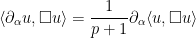
As noted previously, the kinetic energy
 is the Euclidean metric. Indeed, if one assumes that
  are continuously differentiable in both space and time on
 ![{[0,T] \times \mathbf{T}}](https://s0.wp.com/latex.php?latex=%7B%5B0%2CT%5D+%5Ctimes+%5Cmathbf%7BT%7D%7D&bg=ffffff&fg=000000&s=0&c=20201002) , then one can multiply the equation (1) by
, then one can multiply the equation (1) by  and contract against
  to obtain
![{[0,T] \times \mathbf{T}_E}](https://s0.wp.com/latex.php?latex=%7B%5B0%2CT%5D+%5Ctimes+%5Cmathbf%7BT%7D_E%7D&bg=ffffff&fg=000000&s=0&c=20201002) and uses Stokes’ theorem, one obtains the required energy conservation law
and uses Stokes’ theorem, one obtains the required energy conservation law 
 is not a test function and so one cannot immediately integrate (1) against . And indeed, as we shall soon see, it is now known that once the regularity of
  is low enough, energy can “escape to frequency infinity”, leading to failure of the energy conservation law, a phenomenon known in physics as anomalous energy dissipation.
But what is the precise level of regularity needed in order to for this anomalous energy dissipation to occur? To make this question precise, we need a quantitative notion of regularity. One such measure is given by the Hölder space 


 lies between the space
  of continuous functions and the space
  of continuously differentiable functions, and informally describes a space of functions that is “
 times differentiable” in some sense. The above derivation of the energy conservation law involved the integral
 once
once  . More precisely, one can make
Conjecture 1 (Onsager’s conjecture) Let, and let
.
- (i) If
to the Euler equations (in the Leray form
) obeys the energy conservation law (3).
- (ii) If
, then there exist weak solutions
This conjecture was originally arrived at by Onsager by a somewhat different heuristic derivation; see Remark 7. The numerology is also compatible with that arising from the Kolmogorov theory of turbulence (discussed in this previous post), but we will not discuss this interesting connection further here.
The positive part (i) of Onsager conjecture was established by Constantin, E, and Titi, building upon earlier partial results by Eyink; the proof is a relatively straightforward application of Littlewood-Paley theory, and they were also able to work in larger function spaces than 


In these notes we will first establish (i), then discuss the convex integration method in the original context of the Nash-Kuiper embedding theorem. Before tackling the Onsager conjecture (ii) directly, we discuss a related construction of high-dimensional weak solutions in the Sobolev space 


We thank Phil Isett for some comments and corrections.
I’ve just uploaded to the arXiv my paper “Embedding the Heisenberg group into a bounded dimensional Euclidean space with optimal distortion“, submitted to Revista Matematica Iberoamericana. This paper concerns the extent to which one can accurately embed the metric structure of the Heisenberg group
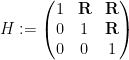
into Euclidean space, which we can write as ![{\{ [x,y,z]: x,y,z \in {\bf R} \}}](https://s0.wp.com/latex.php?latex=%7B%5C%7B+%5Bx%2Cy%2Cz%5D%3A+x%2Cy%2Cz+%5Cin+%7B%5Cbf+R%7D+%5C%7D%7D&bg=ffffff&fg=000000&s=0&c=20201002)
![\displaystyle [x,y,z] := \begin{pmatrix} 1 & x & z \\ 0 & 1 & y \\ 0 & 0 & 1 \end{pmatrix}.](https://s0.wp.com/latex.php?latex=%5Cdisplaystyle+%5Bx%2Cy%2Cz%5D+%3A%3D+%5Cbegin%7Bpmatrix%7D+1+%26+x+%26+z+%5C%5C+0+%26+1+%26+y+%5C%5C+0+%26+0+%26+1+%5Cend%7Bpmatrix%7D.&bg=ffffff&fg=000000&s=0&c=20201002)
Here we give 

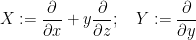
but not from the commutator vector field
![\displaystyle Z := [Y,X] = \frac{\partial}{\partial z}.](https://s0.wp.com/latex.php?latex=%5Cdisplaystyle+Z+%3A%3D+%5BY%2CX%5D+%3D+%5Cfrac%7B%5Cpartial%7D%7B%5Cpartial+z%7D.&bg=ffffff&fg=000000&s=0&c=20201002)
This gives 


On the other hand, if one snowflakes the Heisenberg group by replacing the metric 


Of course, the distortion of this bilipschitz embedding must degenerate in the limit 


The main result of this paper answers this question in the negative:
Theorem 1 There exists an absolute constant
for any
.
To motivate the proof of this theorem, let us first present a bilipschitz map 


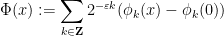
where for each 
and 


with the lower bound

at which point one finds that

as desired.
The key here was that each function 


![{\Gamma := \{ [a,b,c]: a,b,c \in {\bf Z} \}}](https://s0.wp.com/latex.php?latex=%7B%5CGamma+%3A%3D+%5C%7B+%5Ba%2Cb%2Cc%5D%3A+a%2Cb%2Cc+%5Cin+%7B%5Cbf+Z%7D+%5C%7D%7D&bg=ffffff&fg=000000&s=0&c=20201002)


where 
![\displaystyle \delta_\lambda([x,y,z]) := [\lambda x, \lambda y, \lambda^2 z],](https://s0.wp.com/latex.php?latex=%5Cdisplaystyle+%5Cdelta_%5Clambda%28%5Bx%2Cy%2Cz%5D%29+%3A%3D+%5B%5Clambda+x%2C+%5Clambda+y%2C+%5Clambda%5E2+z%5D%2C&bg=ffffff&fg=000000&s=0&c=20201002)
then one can repeat the previous arguments to obtain the required bilipschitz bounds

for the function
To adapt this construction to bounded dimension, the main obstruction was the requirement that the
for all 


One can then try to construct the 


We view this as an underdetermined system of differential equations for 


This problem has some formal similarities with the isometric embedding problem (discussed for instance in this previous post), which can be viewed as the problem of solving an equation of the form 


The isometric embedding problem also has the key obstacle that naive attempts to solve the equation 
To motivate this iteration, we first express 

This reveals that one can construct solutions

for 


To get around this obstacle (which also prominently appears when solving (linearisations of) the isometric embedding equation 

where 


We will construct the low-frequency solution 


To perform the deformation of

of (1) when 


As before, if one directly solves the difference equation (5) using a naive application of (2) with 


and then one can solve (5) by solving the system of equations
for 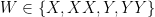
that one would obtain from naively linearising (3) without exploiting the symmetry of 


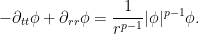
I’ve just uploaded to the arXiv my paper Finite time blowup for a supercritical defocusing nonlinear Schrödinger system, submitted to Analysis and PDE. This paper is an analogue of a recent paper of mine in which I constructed a supercritical defocusing nonlinear wave (NLW) system 

where 


To oversimplify somewhat, the equation (1) is known to be globally regular in the energy-subcritical case when 


in which 
The method of proof in this paper is broadly similar to that in the previous paper for NLW, but with a number of additional technical complications. Both proofs begin by reducing matters to constructing a discretely self-similar solution. In the case of NLW, this solution lived on a forward light cone 

The ability to restrict to a light cone arose from the finite speed of propagation properties of NLW. For NLS, the solution will instead live on the domain

and obey a parabolic self-similarity

and solve the homogeneous version 


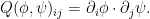
The remaining steps of the argument can broadly be described as quantifier elimination: one systematically eliminates each of the degrees of freedom of the problem in turn by locating the necessary and sufficient conditions required of the remaining degrees of freedom in order for the constraints of a particular degree of freedom to be satisfiable. The first such degree of freedom to eliminate is the potential function 

Firstly, the requirement that

(where 


so if one defines the potential energy field to be 


Conversely, it turns out (roughly speaking) that if one can locate fields 
Now that the potential ![{G[u,u]}](https://s0.wp.com/latex.php?latex=%7BG%5Bu%2Cu%5D%7D&bg=ffffff&fg=000000&s=0&c=20201002)


To eliminate ![{G = G[u,u]}](https://s0.wp.com/latex.php?latex=%7BG+%3D+G%5Bu%2Cu%5D%7D&bg=ffffff&fg=000000&s=0&c=20201002)


and

Ideally one would like a theorem that asserts (for 


After applying the above-mentioned Nash-embedding theorem, the task is now to locate a matrix 


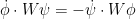
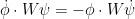
One now has to construct these six fields, together with a potential energy field 
The field 


The potential field 


The task then reduces to locating just two fields 
together with an additional inequality that is the remnant of the momentum conservation law. One can solve for the mass conservation law in terms of a single scalar field

so the problem has finally been simplified to the task of locating a single scalar field
Throughout this post we shall always work in the smooth category, thus all manifolds, maps, coordinate charts, and functions are assumed to be smooth unless explicitly stated otherwise.
A (real) manifold 

Theorem 1 (Whitney embedding theorem) Let
from
In fact, if 


A significant strengthening of the Whitney embedding theorem is (a special case of) the Nash embedding theorem:
Theorem 2 (Nash embedding theorem) Let
In order to obtain the isometric embedding, the dimension

is attained, which I believe is still the record for large 

I recently had the need to invoke the Nash embedding theorem to establish a blowup result for a nonlinear wave equation, which motivated me to go through the proof of the theorem more carefully. Below the fold I give a proof of the theorem that does not attempt to give an optimal value of 


In preparing these notes, I found the articles of Deane Yang and of Siyuan Lu to be helpful.
I’ve just uploaded to the arXiv my paper Finite time blowup for a supercritical defocusing nonlinear wave system, submitted to Analysis and PDE. This paper was inspired by a question asked of me by Sergiu Klainerman recently, regarding whether there were any analogues of my blowup example for Navier-Stokes type equations in the setting of nonlinear wave equations.
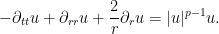
Recall that the defocusing nonlinear wave (NLW) equation reads

where 


where 


Formally, solutions to the equation (2) enjoy a conserved energy
![\displaystyle E[u] = \int_{{\bf R}^d} \frac{1}{2} \|\partial_t u \|^2 + \frac{1}{2} \| \nabla_x u \|^2 + F(u)\ dx.](https://s0.wp.com/latex.php?latex=%5Cdisplaystyle+E%5Bu%5D+%3D+%5Cint_%7B%7B%5Cbf+R%7D%5Ed%7D+%5Cfrac%7B1%7D%7B2%7D+%5C%7C%5Cpartial_t+u+%5C%7C%5E2+%2B+%5Cfrac%7B1%7D%7B2%7D+%5C%7C+%5Cnabla_x+u+%5C%7C%5E2+%2B+F%28u%29%5C+dx.&bg=ffffff&fg=000000&s=0&c=20201002)
Using this conserved energy, it is possible to establish global regularity for the Cauchy problem (2) in the energy-subcritical case when 


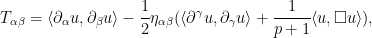
![\displaystyle \int_0^T \int_{{\bf R}^d} \frac{|u(t,x)|^{p+1}}{|x|}\ dx dt \lesssim E[u]](https://s0.wp.com/latex.php?latex=%5Cdisplaystyle+%5Cint_0%5ET+%5Cint_%7B%7B%5Cbf+R%7D%5Ed%7D+%5Cfrac%7B%7Cu%28t%2Cx%29%7C%5E%7Bp%2B1%7D%7D%7B%7Cx%7C%7D%5C+dx+dt+%5Clesssim+E%5Bu%5D+&bg=ffffff&fg=000000&s=0&c=20201002)
which can be proven by manipulating the properties of the stress-energy tensor
(with the usual summation conventions involving the Minkowski metric 

This leaves the question of global regularity for the energy supercritical case when 


Our main result is that finite time blowup can in fact occur, at least for three-dimensional systems where the number
Theorem 1 Let
,
, and
. Then there exists a smooth potential
The rather large lower bound of 
The blowup will in fact be of discrete self-similar type in a backwards light cone, thus
for some fixed 


Because of the discrete self-similarity, the finite time blowup solution will be “locally Type II” in the sense that scale-invariant norms inside the backwards light cone stay bounded as one approaches the singularity. But it will not be “globally Type II” in that scale-invariant norms stay bounded outside the light cone as well; indeed energy will leak from the light cone at every scale. This is consistent with the results of Kenig-Merle and Killip-Visan which preclude “globally Type II” blowup solutions to these equations in many cases.
We now sketch the arguments used to prove this theorem. Usually when studying the NLW, we think of the potential 
Now, one cannot write down a completely arbitrary field

we see that

so the defocusing nature of

Furthermore, taking a derivative of (3) we obtain another constraining equation
that does not explicitly involve the potential

where 
now written in a manner that does not explicitly involve
With this reformulation, this suggests a strategy for locating 


then the question of constructing an (injective) map 

Proposition 2 Let
-manifold, and let
.
Proof: The Nash embedding theorem (in the form given in this ICM lecture of Gunther) shows that 
![{[-R,R]^{19}}](https://s0.wp.com/latex.php?latex=%7B%5B-R%2CR%5D%5E%7B19%7D%7D&bg=ffffff&fg=000000&s=0&c=20201002)

![{[-R,R]}](https://s0.wp.com/latex.php?latex=%7B%5B-R%2CR%5D%7D&bg=ffffff&fg=000000&s=0&c=20201002)


One can presumably improve upon the bound
The remaining task is to construct the stress-energy tensor 

Making the substitution 

(This can be compared with the situation in higher dimensions, in which an undesirable zeroth order term 
and the potential energy density
then one can verify the equation

which can be viewed as a transport equation for 


Recent Comments