Let  be some domain (such as the real numbers). For any natural number
  , let
, let  denote the space of symmetric real-valued functions
  on variables
  , thus

for any permutation  . For instance, for any natural numbers
  , the elementary symmetric polynomials

will be an element of  . With the pointwise product operation, becomes a commutative real algebra. We include the case
  , in which case
  consists solely of the real constants.
Given two natural numbers , one can “lift” a symmetric function  of
of  variables to a symmetric function
 ![{[F^{(k)}]_{k \rightarrow p} \in L(\Omega^p)_{sym}}](https://s0.wp.com/latex.php?latex=%7B%5BF%5E%7B%28k%29%7D%5D_%7Bk+%5Crightarrow+p%7D+%5Cin+L%28%5COmega%5Ep%29_%7Bsym%7D%7D&bg=ffffff&fg=000000&s=0&c=20201002) of variables by the formula
of variables by the formula
![\displaystyle [F^{(k)}]_{k \rightarrow p}(x_1,\dots,x_p) = \sum_{1 \leq i_1 < i_2 < \dots < i_k \leq p} F^{(k)}(x_{i_1}, \dots, x_{i_k})](https://s0.wp.com/latex.php?latex=%5Cdisplaystyle+%5BF%5E%7B%28k%29%7D%5D_%7Bk+%5Crightarrow+p%7D%28x_1%2C%5Cdots%2Cx_p%29+%3D+%5Csum_%7B1+%5Cleq+i_1+%3C+i_2+%3C+%5Cdots+%3C+i_k+%5Cleq+p%7D+F%5E%7B%28k%29%7D%28x_%7Bi_1%7D%2C+%5Cdots%2C+x_%7Bi_k%7D%29+&bg=ffffff&fg=000000&s=0&c=20201002)
where  ranges over all injections from
  to
to  (the latter formula making it clearer that
 ![{[F^{(k)}]_{k \rightarrow p}}](https://s0.wp.com/latex.php?latex=%7B%5BF%5E%7B%28k%29%7D%5D_%7Bk+%5Crightarrow+p%7D%7D&bg=ffffff&fg=000000&s=0&c=20201002) is symmetric). Thus for instance
is symmetric). Thus for instance
![\displaystyle [F^{(1)}(x_1)]_{1 \rightarrow p} = \sum_{i=1}^p F^{(1)}(x_i)](https://s0.wp.com/latex.php?latex=%5Cdisplaystyle+%5BF%5E%7B%281%29%7D%28x_1%29%5D_%7B1+%5Crightarrow+p%7D+%3D+%5Csum_%7Bi%3D1%7D%5Ep+F%5E%7B%281%29%7D%28x_i%29&bg=ffffff&fg=000000&s=0&c=20201002)
![\displaystyle [F^{(2)}(x_1,x_2)]_{2 \rightarrow p} = \sum_{1 \leq i < j \leq p} F^{(2)}(x_i,x_j)](https://s0.wp.com/latex.php?latex=%5Cdisplaystyle+%5BF%5E%7B%282%29%7D%28x_1%2Cx_2%29%5D_%7B2+%5Crightarrow+p%7D+%3D+%5Csum_%7B1+%5Cleq+i+%3C+j+%5Cleq+p%7D+F%5E%7B%282%29%7D%28x_i%2Cx_j%29&bg=ffffff&fg=000000&s=0&c=20201002)
and
![\displaystyle e_k^{(p)}(x_1,\dots,x_p) = [x_1 \dots x_k]_{k \rightarrow p}.](https://s0.wp.com/latex.php?latex=%5Cdisplaystyle+e_k%5E%7B%28p%29%7D%28x_1%2C%5Cdots%2Cx_p%29+%3D+%5Bx_1+%5Cdots+x_k%5D_%7Bk+%5Crightarrow+p%7D.&bg=ffffff&fg=000000&s=0&c=20201002)
Also we have
![\displaystyle [1]_{k \rightarrow p} = \binom{p}{k} = \frac{p(p-1)\dots(p-k+1)}{k!}.](https://s0.wp.com/latex.php?latex=%5Cdisplaystyle+%5B1%5D_%7Bk+%5Crightarrow+p%7D+%3D+%5Cbinom%7Bp%7D%7Bk%7D+%3D+%5Cfrac%7Bp%28p-1%29%5Cdots%28p-k%2B1%29%7D%7Bk%21%7D.&bg=ffffff&fg=000000&s=0&c=20201002)
With these conventions, we see that vanishes for  , and is equal to
  if
if  . We also have the transitivity
![\displaystyle [F^{(k)}]_{k \rightarrow p} = \frac{1}{\binom{p-k}{p-l}} [[F^{(k)}]_{k \rightarrow l}]_{l \rightarrow p}](https://s0.wp.com/latex.php?latex=%5Cdisplaystyle+%5BF%5E%7B%28k%29%7D%5D_%7Bk+%5Crightarrow+p%7D+%3D+%5Cfrac%7B1%7D%7B%5Cbinom%7Bp-k%7D%7Bp-l%7D%7D+%5B%5BF%5E%7B%28k%29%7D%5D_%7Bk+%5Crightarrow+l%7D%5D_%7Bl+%5Crightarrow+p%7D&bg=ffffff&fg=000000&s=0&c=20201002)
if  .
.
The lifting map ![{[]_{k \rightarrow p}}](https://s0.wp.com/latex.php?latex=%7B%5B%5D_%7Bk+%5Crightarrow+p%7D%7D&bg=ffffff&fg=000000&s=0&c=20201002) is a linear map from
is a linear map from  to , but it is not a ring homomorphism. For instance, when
  , one has
![\displaystyle [x_1]_{1 \rightarrow p} [x_1]_{1 \rightarrow p} = (\sum_{i=1}^p x_i)^2 \ \ \ \ \ (1)](https://s0.wp.com/latex.php?latex=%5Cdisplaystyle+%5Bx_1%5D_%7B1+%5Crightarrow+p%7D+%5Bx_1%5D_%7B1+%5Crightarrow+p%7D+%3D+%28%5Csum_%7Bi%3D1%7D%5Ep+x_i%29%5E2+%5C+%5C+%5C+%5C+%5C+%281%29&bg=ffffff&fg=000000&s=0&c=20201002)
![\displaystyle = [x_1^2]_{1 \rightarrow p} + 2 [x_1 x_2]_{1 \rightarrow p}](https://s0.wp.com/latex.php?latex=%5Cdisplaystyle+%3D+%5Bx_1%5E2%5D_%7B1+%5Crightarrow+p%7D+%2B+2+%5Bx_1+x_2%5D_%7B1+%5Crightarrow+p%7D&bg=ffffff&fg=000000&s=0&c=20201002)
![\displaystyle \neq [x_1^2]_{1 \rightarrow p}.](https://s0.wp.com/latex.php?latex=%5Cdisplaystyle+%5Cneq+%5Bx_1%5E2%5D_%7B1+%5Crightarrow+p%7D.&bg=ffffff&fg=000000&s=0&c=20201002)
In general, one has the identity
![\displaystyle [F^{(k)}(x_1,\dots,x_k)]_{k \rightarrow p} [G^{(l)}(x_1,\dots,x_l)]_{l \rightarrow p} = \sum_{k,l \leq m \leq k+l} \frac{1}{k! l!} \ \ \ \ \ (2)](https://s0.wp.com/latex.php?latex=%5Cdisplaystyle+%5BF%5E%7B%28k%29%7D%28x_1%2C%5Cdots%2Cx_k%29%5D_%7Bk+%5Crightarrow+p%7D+%5BG%5E%7B%28l%29%7D%28x_1%2C%5Cdots%2Cx_l%29%5D_%7Bl+%5Crightarrow+p%7D+%3D+%5Csum_%7Bk%2Cl+%5Cleq+m+%5Cleq+k%2Bl%7D+%5Cfrac%7B1%7D%7Bk%21+l%21%7D+%5C+%5C+%5C+%5C+%5C+%282%29&bg=ffffff&fg=000000&s=0&c=20201002)
![\displaystyle [\sum_{\pi, \rho} F^{(k)}(x_{\pi(1)},\dots,x_{\pi(k)}) G^{(l)}(x_{\rho(1)},\dots,x_{\rho(l)})]_{m \rightarrow p}](https://s0.wp.com/latex.php?latex=%5Cdisplaystyle+%5B%5Csum_%7B%5Cpi%2C+%5Crho%7D+F%5E%7B%28k%29%7D%28x_%7B%5Cpi%281%29%7D%2C%5Cdots%2Cx_%7B%5Cpi%28k%29%7D%29+G%5E%7B%28l%29%7D%28x_%7B%5Crho%281%29%7D%2C%5Cdots%2Cx_%7B%5Crho%28l%29%7D%29%5D_%7Bm+%5Crightarrow+p%7D&bg=ffffff&fg=000000&s=0&c=20201002)
for all natural numbers  and ,
and ,  , where
  range over all injections
  ,
,  with
with  . Combinatorially, the identity (2) follows from the fact that given any injections
  and
and  with total image
  of cardinality
  , one has
  , and furthermore there exist precisely
  triples
  of injections , ,
  such that
  and
and  .
.
Example 1 When  , one has
![\displaystyle [x_1 x_2]_{2 \rightarrow p} [x_1]_{1 \rightarrow p} = [\frac{1}{2! 1!}( 2 x_1^2 x_2 + 2 x_1 x_2^2 )]_{2 \rightarrow p} + [\frac{1}{2! 1!} 6 x_1 x_2 x_3]_{3 \rightarrow p}](https://s0.wp.com/latex.php?latex=%5Cdisplaystyle+%5Bx_1+x_2%5D_%7B2+%5Crightarrow+p%7D+%5Bx_1%5D_%7B1+%5Crightarrow+p%7D+%3D+%5B%5Cfrac%7B1%7D%7B2%21+1%21%7D%28+2+x_1%5E2+x_2+%2B+2+x_1+x_2%5E2+%29%5D_%7B2+%5Crightarrow+p%7D+%2B+%5B%5Cfrac%7B1%7D%7B2%21+1%21%7D+6+x_1+x_2+x_3%5D_%7B3+%5Crightarrow+p%7D&bg=ffffff&fg=000000&s=0&c=20201002)
![\displaystyle = [x_1^2 x_2 + x_1 x_2^2]_{2 \rightarrow p} + [3x_1 x_2 x_3]_{3 \rightarrow p}](https://s0.wp.com/latex.php?latex=%5Cdisplaystyle+%3D+%5Bx_1%5E2+x_2+%2B+x_1+x_2%5E2%5D_%7B2+%5Crightarrow+p%7D+%2B+%5B3x_1+x_2+x_3%5D_%7B3+%5Crightarrow+p%7D&bg=ffffff&fg=000000&s=0&c=20201002)
which is just a restatement of the identity

Note that the coefficients appearing in (2) do not depend on the final number of variables . We may therefore abstract the role of from the law (2) by introducing the real algebra  of formal sums
![\displaystyle F^{(*)} = \sum_{k=0}^\infty [F^{(k)}]_{k \rightarrow *}](https://s0.wp.com/latex.php?latex=%5Cdisplaystyle+F%5E%7B%28%2A%29%7D+%3D+%5Csum_%7Bk%3D0%7D%5E%5Cinfty+%5BF%5E%7B%28k%29%7D%5D_%7Bk+%5Crightarrow+%2A%7D&bg=ffffff&fg=000000&s=0&c=20201002)
where for each ,  is an element of (with only finitely many of the being non-zero), and with the formal symbol
 ![{[]_{k \rightarrow *}}](https://s0.wp.com/latex.php?latex=%7B%5B%5D_%7Bk+%5Crightarrow+%2A%7D%7D&bg=ffffff&fg=000000&s=0&c=20201002) being formally linear, thus
being formally linear, thus
![\displaystyle [F^{(k)}]_{k \rightarrow *} + [G^{(k)}]_{k \rightarrow *} := [F^{(k)} + G^{(k)}]_{k \rightarrow *}](https://s0.wp.com/latex.php?latex=%5Cdisplaystyle+%5BF%5E%7B%28k%29%7D%5D_%7Bk+%5Crightarrow+%2A%7D+%2B+%5BG%5E%7B%28k%29%7D%5D_%7Bk+%5Crightarrow+%2A%7D+%3A%3D+%5BF%5E%7B%28k%29%7D+%2B+G%5E%7B%28k%29%7D%5D_%7Bk+%5Crightarrow+%2A%7D&bg=ffffff&fg=000000&s=0&c=20201002)
and
![\displaystyle c [F^{(k)}]_{k \rightarrow *} := [cF^{(k)}]_{k \rightarrow *}](https://s0.wp.com/latex.php?latex=%5Cdisplaystyle+c+%5BF%5E%7B%28k%29%7D%5D_%7Bk+%5Crightarrow+%2A%7D+%3A%3D+%5BcF%5E%7B%28k%29%7D%5D_%7Bk+%5Crightarrow+%2A%7D&bg=ffffff&fg=000000&s=0&c=20201002)
for  and scalars
  , and with multiplication given by the analogue
![\displaystyle [F^{(k)}(x_1,\dots,x_k)]_{k \rightarrow *} [G^{(l)}(x_1,\dots,x_l)]_{l \rightarrow *} = \sum_{k,l \leq m \leq k+l} \frac{1}{k! l!} \ \ \ \ \ (3)](https://s0.wp.com/latex.php?latex=%5Cdisplaystyle+%5BF%5E%7B%28k%29%7D%28x_1%2C%5Cdots%2Cx_k%29%5D_%7Bk+%5Crightarrow+%2A%7D+%5BG%5E%7B%28l%29%7D%28x_1%2C%5Cdots%2Cx_l%29%5D_%7Bl+%5Crightarrow+%2A%7D+%3D+%5Csum_%7Bk%2Cl+%5Cleq+m+%5Cleq+k%2Bl%7D+%5Cfrac%7B1%7D%7Bk%21+l%21%7D+%5C+%5C+%5C+%5C+%5C+%283%29&bg=ffffff&fg=000000&s=0&c=20201002)
![\displaystyle [\sum_{\pi, \rho} F^{(k)}(x_{\pi(1)},\dots,x_{\pi(k)}) G^{(l)}(x_{\rho(1)},\dots,x_{\rho(l)})]_{m \rightarrow *}](https://s0.wp.com/latex.php?latex=%5Cdisplaystyle+%5B%5Csum_%7B%5Cpi%2C+%5Crho%7D+F%5E%7B%28k%29%7D%28x_%7B%5Cpi%281%29%7D%2C%5Cdots%2Cx_%7B%5Cpi%28k%29%7D%29+G%5E%7B%28l%29%7D%28x_%7B%5Crho%281%29%7D%2C%5Cdots%2Cx_%7B%5Crho%28l%29%7D%29%5D_%7Bm+%5Crightarrow+%2A%7D+&bg=ffffff&fg=000000&s=0&c=20201002)
of (2). Thus for instance, in this algebra we have
![\displaystyle [x_1]_{1 \rightarrow *} [x_1]_{1 \rightarrow *} = [x_1^2]_{1 \rightarrow *} + 2 [x_1 x_2]_{2 \rightarrow *}](https://s0.wp.com/latex.php?latex=%5Cdisplaystyle+%5Bx_1%5D_%7B1+%5Crightarrow+%2A%7D+%5Bx_1%5D_%7B1+%5Crightarrow+%2A%7D+%3D+%5Bx_1%5E2%5D_%7B1+%5Crightarrow+%2A%7D+%2B+2+%5Bx_1+x_2%5D_%7B2+%5Crightarrow+%2A%7D&bg=ffffff&fg=000000&s=0&c=20201002)
and
![\displaystyle [x_1 x_2]_{2 \rightarrow *} [x_1]_{1 \rightarrow *} = [x_1^2 x_2 + x_1 x_2^2]_{2 \rightarrow *} + [3 x_1 x_2 x_3]_{3 \rightarrow *}.](https://s0.wp.com/latex.php?latex=%5Cdisplaystyle+%5Bx_1+x_2%5D_%7B2+%5Crightarrow+%2A%7D+%5Bx_1%5D_%7B1+%5Crightarrow+%2A%7D+%3D+%5Bx_1%5E2+x_2+%2B+x_1+x_2%5E2%5D_%7B2+%5Crightarrow+%2A%7D+%2B+%5B3+x_1+x_2+x_3%5D_%7B3+%5Crightarrow+%2A%7D.&bg=ffffff&fg=000000&s=0&c=20201002)
Informally, is an abstraction (or “inverse limit”) of the concept of a symmetric function of an unspecified number of variables, which are formed by summing terms that each involve only a bounded number of these variables at a time. One can check (somewhat tediously) that is indeed a commutative real algebra, with a unit ![{[1]_{0 \rightarrow *}}](https://s0.wp.com/latex.php?latex=%7B%5B1%5D_%7B0+%5Crightarrow+%2A%7D%7D&bg=ffffff&fg=000000&s=0&c=20201002) . (I do not know if this algebra has previously been studied in the literature; it is somewhat analogous to the abstract algebra of finite linear combinations of Schur polynomials, with multiplication given by a Littlewood-Richardson rule. )
. (I do not know if this algebra has previously been studied in the literature; it is somewhat analogous to the abstract algebra of finite linear combinations of Schur polynomials, with multiplication given by a Littlewood-Richardson rule. )
For natural numbers , there is an obvious specialisation map ![{[]_{* \rightarrow p}}](https://s0.wp.com/latex.php?latex=%7B%5B%5D_%7B%2A+%5Crightarrow+p%7D%7D&bg=ffffff&fg=000000&s=0&c=20201002) from to , defined by the formula
from to , defined by the formula
![\displaystyle [\sum_{k=0}^\infty [F^{(k)}]_{k \rightarrow *}]_{* \rightarrow p} := \sum_{k=0}^\infty [F^{(k)}]_{k \rightarrow p}.](https://s0.wp.com/latex.php?latex=%5Cdisplaystyle+%5B%5Csum_%7Bk%3D0%7D%5E%5Cinfty+%5BF%5E%7B%28k%29%7D%5D_%7Bk+%5Crightarrow+%2A%7D%5D_%7B%2A+%5Crightarrow+p%7D+%3A%3D+%5Csum_%7Bk%3D0%7D%5E%5Cinfty+%5BF%5E%7B%28k%29%7D%5D_%7Bk+%5Crightarrow+p%7D.&bg=ffffff&fg=000000&s=0&c=20201002)
Thus, for instance, maps ![{[x_1]_{1 \rightarrow *}}](https://s0.wp.com/latex.php?latex=%7B%5Bx_1%5D_%7B1+%5Crightarrow+%2A%7D%7D&bg=ffffff&fg=000000&s=0&c=20201002) to
to ![{[x_1]_{1 \rightarrow p}}](https://s0.wp.com/latex.php?latex=%7B%5Bx_1%5D_%7B1+%5Crightarrow+p%7D%7D&bg=ffffff&fg=000000&s=0&c=20201002) and
and ![{[x_1 x_2]_{2 \rightarrow *}}](https://s0.wp.com/latex.php?latex=%7B%5Bx_1+x_2%5D_%7B2+%5Crightarrow+%2A%7D%7D&bg=ffffff&fg=000000&s=0&c=20201002) to
to ![{[x_1 x_2]_{2 \rightarrow p}}](https://s0.wp.com/latex.php?latex=%7B%5Bx_1+x_2%5D_%7B2+%5Crightarrow+p%7D%7D&bg=ffffff&fg=000000&s=0&c=20201002) . From (2) and (3) we see that this map
. From (2) and (3) we see that this map ![{[]_{* \rightarrow p}: L(\Omega^*)_{sym} \rightarrow L(\Omega^p)_{sym}}](https://s0.wp.com/latex.php?latex=%7B%5B%5D_%7B%2A+%5Crightarrow+p%7D%3A+L%28%5COmega%5E%2A%29_%7Bsym%7D+%5Crightarrow+L%28%5COmega%5Ep%29_%7Bsym%7D%7D&bg=ffffff&fg=000000&s=0&c=20201002) is an algebra homomorphism, even though the maps
is an algebra homomorphism, even though the maps ![{[]_{k \rightarrow *}: L(\Omega^k)_{sym} \rightarrow L(\Omega^*)_{sym}}](https://s0.wp.com/latex.php?latex=%7B%5B%5D_%7Bk+%5Crightarrow+%2A%7D%3A+L%28%5COmega%5Ek%29_%7Bsym%7D+%5Crightarrow+L%28%5COmega%5E%2A%29_%7Bsym%7D%7D&bg=ffffff&fg=000000&s=0&c=20201002) and
and ![{[]_{k \rightarrow p}: L(\Omega^k)_{sym} \rightarrow L(\Omega^p)_{sym}}](https://s0.wp.com/latex.php?latex=%7B%5B%5D_%7Bk+%5Crightarrow+p%7D%3A+L%28%5COmega%5Ek%29_%7Bsym%7D+%5Crightarrow+L%28%5COmega%5Ep%29_%7Bsym%7D%7D&bg=ffffff&fg=000000&s=0&c=20201002) are not homomorphisms. By inspecting the
are not homomorphisms. By inspecting the  component of we see that the homomorphism is in fact surjective.
Now suppose that we have a measure  on the space , which then induces a product measure
  on every product space
  . To avoid degeneracies we will assume that the integral
  is strictly positive. Assuming suitable measurability and integrability hypotheses, a function
  can then be integrated against this product measure to produce a number

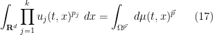
In the event that arises as a lift of another function , then from Fubini’s theorem we obtain the formula
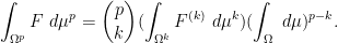
Thus for instance, if ,
![\displaystyle \int_{{\bf R}^p} [x_1]_{1 \rightarrow p}\ d\mu^p = p (\int_{\bf R} x\ d\mu(x)) (\int_{\bf R} \mu)^{p-1} \ \ \ \ \ (4)](https://s0.wp.com/latex.php?latex=%5Cdisplaystyle+%5Cint_%7B%7B%5Cbf+R%7D%5Ep%7D+%5Bx_1%5D_%7B1+%5Crightarrow+p%7D%5C+d%5Cmu%5Ep+%3D+p+%28%5Cint_%7B%5Cbf+R%7D+x%5C+d%5Cmu%28x%29%29+%28%5Cint_%7B%5Cbf+R%7D+%5Cmu%29%5E%7Bp-1%7D+%5C+%5C+%5C+%5C+%5C+%284%29&bg=ffffff&fg=000000&s=0&c=20201002)
and
![\displaystyle \int_{{\bf R}^p} [x_1 x_2]_{2 \rightarrow p}\ d\mu^p = \binom{p}{2} (\int_{{\bf R}^2} x_1 x_2\ d\mu(x_1) d\mu(x_2)) (\int_{\bf R} \mu)^{p-2}. \ \ \ \ \ (5)](https://s0.wp.com/latex.php?latex=%5Cdisplaystyle+%5Cint_%7B%7B%5Cbf+R%7D%5Ep%7D+%5Bx_1+x_2%5D_%7B2+%5Crightarrow+p%7D%5C+d%5Cmu%5Ep+%3D+%5Cbinom%7Bp%7D%7B2%7D+%28%5Cint_%7B%7B%5Cbf+R%7D%5E2%7D+x_1+x_2%5C+d%5Cmu%28x_1%29+d%5Cmu%28x_2%29%29+%28%5Cint_%7B%5Cbf+R%7D+%5Cmu%29%5E%7Bp-2%7D.+%5C+%5C+%5C+%5C+%5C+%285%29&bg=ffffff&fg=000000&s=0&c=20201002)
On summing, we see that if
is an element of the formal algebra , then
![\displaystyle \int_{\Omega^p} [F^{(*)}]_{* \rightarrow p}\ d\mu^p = \sum_{k=0}^\infty \binom{p}{k} (\int_{\Omega^k} F^{(k)}\ d\mu^k) (\int_\Omega\ d\mu)^{p-k}. \ \ \ \ \ (6)](https://s0.wp.com/latex.php?latex=%5Cdisplaystyle+%5Cint_%7B%5COmega%5Ep%7D+%5BF%5E%7B%28%2A%29%7D%5D_%7B%2A+%5Crightarrow+p%7D%5C+d%5Cmu%5Ep+%3D+%5Csum_%7Bk%3D0%7D%5E%5Cinfty+%5Cbinom%7Bp%7D%7Bk%7D+%28%5Cint_%7B%5COmega%5Ek%7D+F%5E%7B%28k%29%7D%5C+d%5Cmu%5Ek%29+%28%5Cint_%5COmega%5C+d%5Cmu%29%5E%7Bp-k%7D.+%5C+%5C+%5C+%5C+%5C+%286%29&bg=ffffff&fg=000000&s=0&c=20201002)
Note that by hypothesis, only finitely many terms on the right-hand side are non-zero.
Now for a key observation: whereas the left-hand side of (6) only makes sense when is a natural number, the right-hand side is meaningful when takes a fractional value (or even when it takes negative or complex values!), interpreting the binomial coefficient  as a polynomial
  in . As such, this suggests a way to introduce a “virtual” concept of a symmetric function on a fractional power space for such values of , and even to integrate such functions against product measures , even if the fractional power does not exist in the usual set-theoretic sense (and similarly does not exist in the usual measure-theoretic sense). More precisely, for arbitrary real or complex , we now define to be the space of abstract objects
![\displaystyle F^{(p)} = [F^{(*)}]_{* \rightarrow p} = \sum_{k=0}^\infty [F^{(k)}]_{k \rightarrow p}](https://s0.wp.com/latex.php?latex=%5Cdisplaystyle+F%5E%7B%28p%29%7D+%3D+%5BF%5E%7B%28%2A%29%7D%5D_%7B%2A+%5Crightarrow+p%7D+%3D+%5Csum_%7Bk%3D0%7D%5E%5Cinfty+%5BF%5E%7B%28k%29%7D%5D_%7Bk+%5Crightarrow+p%7D&bg=ffffff&fg=000000&s=0&c=20201002)
with  and (and now interpreted as formal symbols, with the structure of a commutative real algebra inherited from , thus
![\displaystyle [F^{(*)}]_{* \rightarrow p} + [G^{(*)}]_{* \rightarrow p} := [F^{(*)} + G^{(*)}]_{* \rightarrow p}](https://s0.wp.com/latex.php?latex=%5Cdisplaystyle+%5BF%5E%7B%28%2A%29%7D%5D_%7B%2A+%5Crightarrow+p%7D+%2B+%5BG%5E%7B%28%2A%29%7D%5D_%7B%2A+%5Crightarrow+p%7D+%3A%3D+%5BF%5E%7B%28%2A%29%7D+%2B+G%5E%7B%28%2A%29%7D%5D_%7B%2A+%5Crightarrow+p%7D&bg=ffffff&fg=000000&s=0&c=20201002)
![\displaystyle c [F^{(*)}]_{* \rightarrow p} := [c F^{(*)}]_{* \rightarrow p}](https://s0.wp.com/latex.php?latex=%5Cdisplaystyle+c+%5BF%5E%7B%28%2A%29%7D%5D_%7B%2A+%5Crightarrow+p%7D+%3A%3D+%5Bc+F%5E%7B%28%2A%29%7D%5D_%7B%2A+%5Crightarrow+p%7D&bg=ffffff&fg=000000&s=0&c=20201002)
![\displaystyle [F^{(*)}]_{* \rightarrow p} [G^{(*)}]_{* \rightarrow p} := [F^{(*)} G^{(*)}]_{* \rightarrow p}.](https://s0.wp.com/latex.php?latex=%5Cdisplaystyle+%5BF%5E%7B%28%2A%29%7D%5D_%7B%2A+%5Crightarrow+p%7D+%5BG%5E%7B%28%2A%29%7D%5D_%7B%2A+%5Crightarrow+p%7D+%3A%3D+%5BF%5E%7B%28%2A%29%7D+G%5E%7B%28%2A%29%7D%5D_%7B%2A+%5Crightarrow+p%7D.&bg=ffffff&fg=000000&s=0&c=20201002)
In particular, the multiplication law (2) continues to hold for such values of , thanks to (3). Given any measure on , we formally define a measure on with regards to which we can integrate elements  of by the formula (6) (providing one has sufficient measurability and integrability to make sense of this formula), thus providing a sort of “fractional dimensional integral” for symmetric functions. Thus, for instance, with this formalism the identities (4), (5) now hold for fractional values of , even though the formal space
  no longer makes sense as a set, and the formal measure no longer makes sense as a measure. (The formalism here is somewhat reminiscent of the technique of dimensional regularisation employed in the physical literature in order to assign values to otherwise divergent integrals. See also this post for an unrelated abstraction of the integration concept involving integration over supercommutative variables (and in particular over fermionic variables).)
Example 2 Suppose is a probability measure on , and  is a random variable; on any power
  , we let
  be the usual independent copies of
  on , thus
  for
for  . Then for any real or complex , the formal integral
![\displaystyle \int_{\Omega^p} [X_1]_{1 \rightarrow p}^2\ d\mu^p](https://s0.wp.com/latex.php?latex=%5Cdisplaystyle+%5Cint_%7B%5COmega%5Ep%7D+%5BX_1%5D_%7B1+%5Crightarrow+p%7D%5E2%5C+d%5Cmu%5Ep+&bg=ffffff&fg=000000&s=0&c=20201002)
can be evaluated by first using the identity
![\displaystyle [X_1]_{1 \rightarrow p}^2 = [X_1^2]_{1 \rightarrow p} + 2[X_1 X_2]_{2 \rightarrow p}](https://s0.wp.com/latex.php?latex=%5Cdisplaystyle+%5BX_1%5D_%7B1+%5Crightarrow+p%7D%5E2+%3D+%5BX_1%5E2%5D_%7B1+%5Crightarrow+p%7D+%2B+2%5BX_1+X_2%5D_%7B2+%5Crightarrow+p%7D&bg=ffffff&fg=000000&s=0&c=20201002)
(cf. (1)) and then using (6) and the probability measure hypothesis  to conclude that
![\displaystyle \int_{\Omega^p} [X_1]_{1 \rightarrow p}^2\ d\mu^p = \binom{p}{1} \int_{\Omega} X^2\ d\mu + 2 \binom{p}{2} \int_{\Omega^2} X_1 X_2\ d\mu^2](https://s0.wp.com/latex.php?latex=%5Cdisplaystyle+%5Cint_%7B%5COmega%5Ep%7D+%5BX_1%5D_%7B1+%5Crightarrow+p%7D%5E2%5C+d%5Cmu%5Ep+%3D+%5Cbinom%7Bp%7D%7B1%7D+%5Cint_%7B%5COmega%7D+X%5E2%5C+d%5Cmu+%2B+2+%5Cbinom%7Bp%7D%7B2%7D+%5Cint_%7B%5COmega%5E2%7D+X_1+X_2%5C+d%5Cmu%5E2&bg=ffffff&fg=000000&s=0&c=20201002)

or in probabilistic notation
![\displaystyle \int_{\Omega^p} [X_1]_{1 \rightarrow p}^2\ d\mu^p = p \mathbf{Var}(X) + p^2 \mathbf{E}(X)^2. \ \ \ \ \ (7)](https://s0.wp.com/latex.php?latex=%5Cdisplaystyle+%5Cint_%7B%5COmega%5Ep%7D+%5BX_1%5D_%7B1+%5Crightarrow+p%7D%5E2%5C+d%5Cmu%5Ep+%3D+p+%5Cmathbf%7BVar%7D%28X%29+%2B+p%5E2+%5Cmathbf%7BE%7D%28X%29%5E2.+%5C+%5C+%5C+%5C+%5C+%287%29&bg=ffffff&fg=000000&s=0&c=20201002)
For a natural number, this identity has the probabilistic interpretation

whenever  are jointly independent copies of , which reflects the well known fact that the sum
  has expectation
  and variance
  . One can thus view (7) as an abstract generalisation of (8) to the case when is fractional, negative, or even complex, despite the fact that there is no sensible way in this case to talk about independent copies of in the standard framework of probability theory.
In this particular case, the quantity (7) is non-negative for every nonnegative , which looks plausible given the form of the left-hand side. Unfortunately, this sort of non-negativity does not always hold; for instance, if has mean zero, one can check that
![\displaystyle \int_{\Omega^p} [X_1]_{1 \rightarrow p}^4\ d\mu^p = p \mathbf{Var}(X^2) + p(3p-2) (\mathbf{E}(X^2))^2](https://s0.wp.com/latex.php?latex=%5Cdisplaystyle+%5Cint_%7B%5COmega%5Ep%7D+%5BX_1%5D_%7B1+%5Crightarrow+p%7D%5E4%5C+d%5Cmu%5Ep+%3D+p+%5Cmathbf%7BVar%7D%28X%5E2%29+%2B+p%283p-2%29+%28%5Cmathbf%7BE%7D%28X%5E2%29%29%5E2&bg=ffffff&fg=000000&s=0&c=20201002)
and the right-hand side can become negative for  . This is a shame, because otherwise one could hope to start endowing
  with some sort of commutative von Neumann algebra type structure (or the abstract probability structure discussed in this previous post) and then interpret it as a genuine measure space rather than as a virtual one. (This failure of positivity is related to the fact that the characteristic function of a random variable, when raised to the power, need not be a characteristic function of any random variable once is no longer a natural number: “fractional convolution” does not preserve positivity!) However, one vestige of positivity remains: if
  is non-negative, then so is
![\displaystyle \int_{\Omega^p} [F]_{1 \rightarrow p}\ d\mu^p = p (\int_\Omega F\ d\mu) (\int_\Omega\ d\mu)^{p-1}.](https://s0.wp.com/latex.php?latex=%5Cdisplaystyle+%5Cint_%7B%5COmega%5Ep%7D+%5BF%5D_%7B1+%5Crightarrow+p%7D%5C+d%5Cmu%5Ep+%3D+p+%28%5Cint_%5COmega+F%5C+d%5Cmu%29+%28%5Cint_%5COmega%5C+d%5Cmu%29%5E%7Bp-1%7D.&bg=ffffff&fg=000000&s=0&c=20201002)
One can wonder what the point is to all of this abstract formalism and how it relates to the rest of mathematics. For me, this formalism originated implicitly in an old paper I wrote with Jon Bennett and Tony Carbery on the multilinear restriction and Kakeya conjectures, though we did not have a good language for working with it at the time, instead working first with the case of natural number exponents and appealing to a general extrapolation theorem to then obtain various identities in the fractional case. The connection between these fractional dimensional integrals and more traditional integrals ultimately arises from the simple identity

(where the right-hand side should be viewed as the fractional dimensional integral of the unit ![{[1]_{0 \rightarrow p}}](https://s0.wp.com/latex.php?latex=%7B%5B1%5D_%7B0+%5Crightarrow+p%7D%7D&bg=ffffff&fg=000000&s=0&c=20201002) against ). As such, one can manipulate powers of ordinary integrals using the machinery of fractional dimensional integrals. A key lemma in this regard is
against ). As such, one can manipulate powers of ordinary integrals using the machinery of fractional dimensional integrals. A key lemma in this regard is
Lemma 3 (Differentiation formula) Suppose that a positive measure  on depends on some parameter
  and varies by the formula

for some function  . Let be any real or complex number. Then, assuming sufficient smoothness and integrability of all quantities involved, we have
![\displaystyle \frac{d}{dt} \int_{\Omega^p} F^{(p)}\ d\mu(t)^p = \int_{\Omega^p} F^{(p)} [a(t)]_{1 \rightarrow p}\ d\mu(t)^p \ \ \ \ \ (10)](https://s0.wp.com/latex.php?latex=%5Cdisplaystyle+%5Cfrac%7Bd%7D%7Bdt%7D+%5Cint_%7B%5COmega%5Ep%7D+F%5E%7B%28p%29%7D%5C+d%5Cmu%28t%29%5Ep+%3D+%5Cint_%7B%5COmega%5Ep%7D+F%5E%7B%28p%29%7D+%5Ba%28t%29%5D_%7B1+%5Crightarrow+p%7D%5C+d%5Cmu%28t%29%5Ep+%5C+%5C+%5C+%5C+%5C+%2810%29&bg=ffffff&fg=000000&s=0&c=20201002)
for all  that are independent of . If we allow
  to now depend on also, then we have the more general total derivative formula

![\displaystyle = \int_{\Omega^p} \frac{d}{dt} F^{(p)}(t) + F^{(p)}(t) [a(t)]_{1 \rightarrow p}\ d\mu(t)^p,](https://s0.wp.com/latex.php?latex=%5Cdisplaystyle+%3D+%5Cint_%7B%5COmega%5Ep%7D+%5Cfrac%7Bd%7D%7Bdt%7D+F%5E%7B%28p%29%7D%28t%29+%2B+F%5E%7B%28p%29%7D%28t%29+%5Ba%28t%29%5D_%7B1+%5Crightarrow+p%7D%5C+d%5Cmu%28t%29%5Ep%2C+&bg=ffffff&fg=000000&s=0&c=20201002)
again assuming sufficient amounts of smoothness and regularity.
Proof: We just prove (10), as (11) then follows by same argument used to prove the usual product rule. By linearity it suffices to verify this identity in the case ![{F^{(p)} = [F^{(k)}]_{k \rightarrow p}}](https://s0.wp.com/latex.php?latex=%7BF%5E%7B%28p%29%7D+%3D+%5BF%5E%7B%28k%29%7D%5D_%7Bk+%5Crightarrow+p%7D%7D&bg=ffffff&fg=000000&s=0&c=20201002) for some symmetric function for a natural number . By (6), the left-hand side of (10) is then
for some symmetric function for a natural number . By (6), the left-hand side of (10) is then
![\displaystyle \frac{d}{dt} [\binom{p}{k} (\int_{\Omega^k} F^{(k)}\ d\mu(t)^k) (\int_\Omega\ d\mu(t))^{p-k}]. \ \ \ \ \ (12)](https://s0.wp.com/latex.php?latex=%5Cdisplaystyle+%5Cfrac%7Bd%7D%7Bdt%7D+%5B%5Cbinom%7Bp%7D%7Bk%7D+%28%5Cint_%7B%5COmega%5Ek%7D+F%5E%7B%28k%29%7D%5C+d%5Cmu%28t%29%5Ek%29+%28%5Cint_%5COmega%5C+d%5Cmu%28t%29%29%5E%7Bp-k%7D%5D.+%5C+%5C+%5C+%5C+%5C+%2812%29&bg=ffffff&fg=000000&s=0&c=20201002)
Differentiating under the integral sign using (9) we have
and similarly

where  are the standard copies of
  on :
on :
By the product rule, we can thus expand (12) as
where we have suppressed the dependence on for brevity. Since  , we can write this expression using (6) as
![\displaystyle \int_{\Omega^p} [F^{(k)} (a_1 + \dots + a_k)]_{k \rightarrow p} + [ F^{(k)} \ast a ]_{k+1 \rightarrow p}\ d\mu^p](https://s0.wp.com/latex.php?latex=%5Cdisplaystyle+%5Cint_%7B%5COmega%5Ep%7D+%5BF%5E%7B%28k%29%7D+%28a_1+%2B+%5Cdots+%2B+a_k%29%5D_%7Bk+%5Crightarrow+p%7D+%2B+%5B+F%5E%7B%28k%29%7D+%5Cast+a+%5D_%7Bk%2B1+%5Crightarrow+p%7D%5C+d%5Cmu%5Ep&bg=ffffff&fg=000000&s=0&c=20201002)
where  is the symmetric function

But from (2) one has
![\displaystyle [F^{(k)} (a_1 + \dots + a_k)]_{k \rightarrow p} + [ F^{(k)} \ast a ]_{k+1 \rightarrow p} = [F^{(k)}]_{k \rightarrow p} [a]_{1 \rightarrow p}](https://s0.wp.com/latex.php?latex=%5Cdisplaystyle+%5BF%5E%7B%28k%29%7D+%28a_1+%2B+%5Cdots+%2B+a_k%29%5D_%7Bk+%5Crightarrow+p%7D+%2B+%5B+F%5E%7B%28k%29%7D+%5Cast+a+%5D_%7Bk%2B1+%5Crightarrow+p%7D+%3D+%5BF%5E%7B%28k%29%7D%5D_%7Bk+%5Crightarrow+p%7D+%5Ba%5D_%7B1+%5Crightarrow+p%7D&bg=ffffff&fg=000000&s=0&c=20201002)
and the claim follows. 
Remark 4 It is also instructive to prove this lemma in the special case when is a natural number, in which case the fractional dimensional integral  can be interpreted as a classical integral. In this case, the identity (10) is immediate from applying the product rule to (9) to conclude that
![\displaystyle \frac{d}{dt} d\mu(t)^p = [a(t)]_{1 \rightarrow p} d\mu(t)^p.](https://s0.wp.com/latex.php?latex=%5Cdisplaystyle+%5Cfrac%7Bd%7D%7Bdt%7D+d%5Cmu%28t%29%5Ep+%3D+%5Ba%28t%29%5D_%7B1+%5Crightarrow+p%7D+d%5Cmu%28t%29%5Ep.&bg=ffffff&fg=000000&s=0&c=20201002)
One could in fact derive (10) for arbitrary real or complex from the case when is a natural number by an extrapolation argument; see the appendix of my paper with Bennett and Carbery for details.
Let us give a simple PDE application of this lemma as illustration:
Proposition 5 (Heat flow monotonicity) Let  be a solution to the heat equation
  with initial data
  a rapidly decreasing finite non-negative Radon measure, or more explicitly

for al  . Then for any
  , the quantity

is monotone non-decreasing in  for
for  , constant for
  , and monotone non-increasing for
  .
.
Proof: By a limiting argument we may assume that  is absolutely continuous, with Radon-Nikodym derivative a test function; this is more than enough regularity to justify the arguments below.
For any  , let
, let  denote the Radon measure
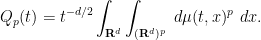
Then the quantity  can be written as a fractional dimensional integral
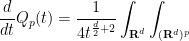
Observe that

and thus by Lemma 3 and the product rule
![\displaystyle \frac{d}{dt} Q_p(t) = -\frac{d}{2t} Q_p(t) + t^{-d/2} \int_{{\bf R}^d} \int_{({\bf R}^d)^p} [\frac{|x-y|^2}{4t^2}]_{1 \rightarrow p} d\mu(t,x)^p\ dx \ \ \ \ \ (13)](https://s0.wp.com/latex.php?latex=%5Cdisplaystyle+%5Cfrac%7Bd%7D%7Bdt%7D+Q_p%28t%29+%3D+-%5Cfrac%7Bd%7D%7B2t%7D+Q_p%28t%29+%2B+t%5E%7B-d%2F2%7D+%5Cint_%7B%7B%5Cbf+R%7D%5Ed%7D+%5Cint_%7B%28%7B%5Cbf+R%7D%5Ed%29%5Ep%7D+%5B%5Cfrac%7B%7Cx-y%7C%5E2%7D%7B4t%5E2%7D%5D_%7B1+%5Crightarrow+p%7D+d%5Cmu%28t%2Cx%29%5Ep%5C+dx+%5C+%5C+%5C+%5C+%5C+%2813%29&bg=ffffff&fg=000000&s=0&c=20201002)
where we use  for the variable of integration in the factor space
  of
of  .
.
To simplify this expression we will take advantage of integration by parts in the  variable. Specifically, in any direction
  , we have
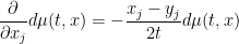
and hence by Lemma 3
![\displaystyle \frac{\partial}{\partial x_j} \int_{({\bf R}^d)^p}\ d\mu(t,x)^p\ dx = - \int_{({\bf R}^d)^p} [\frac{x_j-y_j}{2t}]_{1 \rightarrow p}\ d\mu(t,x)^p\ dx.](https://s0.wp.com/latex.php?latex=%5Cdisplaystyle+%5Cfrac%7B%5Cpartial%7D%7B%5Cpartial+x_j%7D+%5Cint_%7B%28%7B%5Cbf+R%7D%5Ed%29%5Ep%7D%5C+d%5Cmu%28t%2Cx%29%5Ep%5C+dx+%3D+-+%5Cint_%7B%28%7B%5Cbf+R%7D%5Ed%29%5Ep%7D+%5B%5Cfrac%7Bx_j-y_j%7D%7B2t%7D%5D_%7B1+%5Crightarrow+p%7D%5C+d%5Cmu%28t%2Cx%29%5Ep%5C+dx.&bg=ffffff&fg=000000&s=0&c=20201002)
Multiplying by and integrating by parts, we see that
![\displaystyle d Q_p(t) = \int_{{\bf R}^d} \int_{({\bf R}^d)^p} x_j [\frac{x_j-y_j}{2t}]_{1 \rightarrow p}\ d\mu(t,x)^p\ dx](https://s0.wp.com/latex.php?latex=%5Cdisplaystyle+d+Q_p%28t%29+%3D+%5Cint_%7B%7B%5Cbf+R%7D%5Ed%7D+%5Cint_%7B%28%7B%5Cbf+R%7D%5Ed%29%5Ep%7D+x_j+%5B%5Cfrac%7Bx_j-y_j%7D%7B2t%7D%5D_%7B1+%5Crightarrow+p%7D%5C+d%5Cmu%28t%2Cx%29%5Ep%5C+dx&bg=ffffff&fg=000000&s=0&c=20201002)
![\displaystyle = \int_{{\bf R}^d} \int_{({\bf R}^d)^p} x_j [\frac{x_j-y_j}{2t}]_{1 \rightarrow p}\ d\mu(t,x)^p\ dx](https://s0.wp.com/latex.php?latex=%5Cdisplaystyle+%3D+%5Cint_%7B%7B%5Cbf+R%7D%5Ed%7D+%5Cint_%7B%28%7B%5Cbf+R%7D%5Ed%29%5Ep%7D+x_j+%5B%5Cfrac%7Bx_j-y_j%7D%7B2t%7D%5D_%7B1+%5Crightarrow+p%7D%5C+d%5Cmu%28t%2Cx%29%5Ep%5C+dx&bg=ffffff&fg=000000&s=0&c=20201002)
where we use the Einstein summation convention in  . Similarly, if
  is any reasonable function depending only on , we have
![\displaystyle \frac{\partial}{\partial x_j} \int_{({\bf R}^d)^p}[F_j(y)]_{1 \rightarrow p}\ d\mu(t,x)^p\ dx](https://s0.wp.com/latex.php?latex=%5Cdisplaystyle+%5Cfrac%7B%5Cpartial%7D%7B%5Cpartial+x_j%7D+%5Cint_%7B%28%7B%5Cbf+R%7D%5Ed%29%5Ep%7D%5BF_j%28y%29%5D_%7B1+%5Crightarrow+p%7D%5C+d%5Cmu%28t%2Cx%29%5Ep%5C+dx+&bg=ffffff&fg=000000&s=0&c=20201002)
![\displaystyle = - \int_{({\bf R}^d)^p} [F_j(y)]_{1 \rightarrow p} [\frac{x_j-y_j}{2t}]_{1 \rightarrow p}\ d\mu(t,x)^p\ dx](https://s0.wp.com/latex.php?latex=%5Cdisplaystyle+%3D+-+%5Cint_%7B%28%7B%5Cbf+R%7D%5Ed%29%5Ep%7D+%5BF_j%28y%29%5D_%7B1+%5Crightarrow+p%7D+%5B%5Cfrac%7Bx_j-y_j%7D%7B2t%7D%5D_%7B1+%5Crightarrow+p%7D%5C+d%5Cmu%28t%2Cx%29%5Ep%5C+dx&bg=ffffff&fg=000000&s=0&c=20201002)
and hence on integration by parts
![\displaystyle 0 = \int_{{\bf R}^d} \int_{({\bf R}^d)^p} [F_j(y) \frac{x_j-y_j}{2t}]_{1 \rightarrow p}\ d\mu(t,x)^p\ dx.](https://s0.wp.com/latex.php?latex=%5Cdisplaystyle+0+%3D+%5Cint_%7B%7B%5Cbf+R%7D%5Ed%7D+%5Cint_%7B%28%7B%5Cbf+R%7D%5Ed%29%5Ep%7D+%5BF_j%28y%29+%5Cfrac%7Bx_j-y_j%7D%7B2t%7D%5D_%7B1+%5Crightarrow+p%7D%5C+d%5Cmu%28t%2Cx%29%5Ep%5C+dx.&bg=ffffff&fg=000000&s=0&c=20201002)
We conclude that
![\displaystyle \frac{d}{2t} Q_p(t) = t^{-d/2} \int_{{\bf R}^d} \int_{({\bf R}^d)^p} (x_j - [F_j(y)]_{1 \rightarrow p}) [\frac{(x_j-y_j)}{4t}]_{1 \rightarrow p} d\mu(t,x)^p\ dx](https://s0.wp.com/latex.php?latex=%5Cdisplaystyle+%5Cfrac%7Bd%7D%7B2t%7D+Q_p%28t%29+%3D+t%5E%7B-d%2F2%7D+%5Cint_%7B%7B%5Cbf+R%7D%5Ed%7D+%5Cint_%7B%28%7B%5Cbf+R%7D%5Ed%29%5Ep%7D+%28x_j+-+%5BF_j%28y%29%5D_%7B1+%5Crightarrow+p%7D%29+%5B%5Cfrac%7B%28x_j-y_j%29%7D%7B4t%7D%5D_%7B1+%5Crightarrow+p%7D+d%5Cmu%28t%2Cx%29%5Ep%5C+dx+&bg=ffffff&fg=000000&s=0&c=20201002)
and thus by (13)
![\displaystyle [(x_j-y_j)(x_j-y_j)]_{1 \rightarrow p} - (x_j - [F_j(y)]_{1 \rightarrow p}) [x_j - y_j]_{1 \rightarrow p}\ d\mu(t,x)^p\ dx.](https://s0.wp.com/latex.php?latex=%5Cdisplaystyle+%5B%28x_j-y_j%29%28x_j-y_j%29%5D_%7B1+%5Crightarrow+p%7D+-+%28x_j+-+%5BF_j%28y%29%5D_%7B1+%5Crightarrow+p%7D%29+%5Bx_j+-+y_j%5D_%7B1+%5Crightarrow+p%7D%5C+d%5Cmu%28t%2Cx%29%5Ep%5C+dx.&bg=ffffff&fg=000000&s=0&c=20201002)
The choice of  that then achieves the most cancellation turns out to be
  (this cancels the terms that are linear or quadratic in the ), so that
 ![{x_j - [F_j(y)]_{1 \rightarrow p} = \frac{1}{p} [x_j - y_j]_{1 \rightarrow p}}](https://s0.wp.com/latex.php?latex=%7Bx_j+-+%5BF_j%28y%29%5D_%7B1+%5Crightarrow+p%7D+%3D+%5Cfrac%7B1%7D%7Bp%7D+%5Bx_j+-+y_j%5D_%7B1+%5Crightarrow+p%7D%7D&bg=ffffff&fg=000000&s=0&c=20201002) . Repeating the calculations establishing (7), one has
. Repeating the calculations establishing (7), one has
![\displaystyle \int_{({\bf R}^d)^p} [(x_j-y_j)(x_j-y_j)]_{1 \rightarrow p}\ d\mu^p = p \mathop{\bf E} |x-Y|^2 (\int_{{\bf R}^d}\ d\mu)^{p}](https://s0.wp.com/latex.php?latex=%5Cdisplaystyle+%5Cint_%7B%28%7B%5Cbf+R%7D%5Ed%29%5Ep%7D+%5B%28x_j-y_j%29%28x_j-y_j%29%5D_%7B1+%5Crightarrow+p%7D%5C+d%5Cmu%5Ep+%3D+p+%5Cmathop%7B%5Cbf+E%7D+%7Cx-Y%7C%5E2+%28%5Cint_%7B%7B%5Cbf+R%7D%5Ed%7D%5C+d%5Cmu%29%5E%7Bp%7D&bg=ffffff&fg=000000&s=0&c=20201002)
and
![\displaystyle \int_{({\bf R}^d)^p} [x_j-y_j]_{1 \rightarrow p} [x_j-y_j]_{1 \rightarrow p}\ d\mu^p](https://s0.wp.com/latex.php?latex=%5Cdisplaystyle+%5Cint_%7B%28%7B%5Cbf+R%7D%5Ed%29%5Ep%7D+%5Bx_j-y_j%5D_%7B1+%5Crightarrow+p%7D+%5Bx_j-y_j%5D_%7B1+%5Crightarrow+p%7D%5C+d%5Cmu%5Ep+&bg=ffffff&fg=000000&s=0&c=20201002)

where  is the random variable drawn from with the normalised probability measure
  . Since
  , one thus has

This expression is clearly non-negative for  , equal to zero for , and positive for , giving the claim. (One could simplify
  here as
  if desired, though it is not strictly necessary to do so for the proof.)
Remark 6 As with Remark 4, one can also establish the identity (14) first for natural numbers by direct computation avoiding the theory of fractional dimensional integrals, and then extrapolate to the case of more general values of . This particular identity is also simple enough that it can be directly established by integration by parts without much difficulty, even for fractional values of .
A more complicated version of this argument establishes the non-endpoint multilinear Kakeya inequality (without any logarithmic loss in a scale parameter  ); this was established in my previous paper with Jon Bennett and Tony Carbery, but using the “natural number first” approach rather than using the current formalism of fractional dimensional integration. However, the arguments can be translated into this formalism without much difficulty; we do so below the fold. (To simplify the exposition slightly we will not address issues of establishing enough regularity and integrability to justify all the manipulations, though in practice this can be done by standard limiting arguments.)
— 1. Multilinear heat flow monotonicity —
Before we give a multilinear variant of Proposition 5 of relevance to the multilinear Kakeya inequality, we first need to briefly set up the theory of finite products
of fractional powers of spaces  , where
  are real or complex numbers. The functions
  to integrate here lie in the tensor product space

which is generated by tensor powers
with  , with the usual tensor product identifications and algebra operations. One can evaluate fractional dimensional integrals of such functions against “virtual product measures”
  , with
  a measure on
  , by the natural formula

assuming sufficient measurability and integrability hypotheses. We can lift functions  to an element
 ![{[F_j^{(m)}]_{m \rightarrow p; j}}](https://s0.wp.com/latex.php?latex=%7B%5BF_j%5E%7B%28m%29%7D%5D_%7Bm+%5Crightarrow+p%3B+j%7D%7D&bg=ffffff&fg=000000&s=0&c=20201002) of the space (15) by the formula
of the space (15) by the formula
![\displaystyle [F_j^{(m)}]_{m \rightarrow p; j} := 1^{\otimes j-1} \otimes [F_j^{(m)}]_{m \rightarrow p} \otimes 1^{\otimes k-j}.](https://s0.wp.com/latex.php?latex=%5Cdisplaystyle+%5BF_j%5E%7B%28m%29%7D%5D_%7Bm+%5Crightarrow+p%3B+j%7D+%3A%3D+1%5E%7B%5Cotimes+j-1%7D+%5Cotimes+%5BF_j%5E%7B%28m%29%7D%5D_%7Bm+%5Crightarrow+p%7D+%5Cotimes+1%5E%7B%5Cotimes+k-j%7D.&bg=ffffff&fg=000000&s=0&c=20201002)
This is easily seen to be an algebra homomorphism.
Example 7 If  and
and  are functions and
  are measures on
  respectively, then (assuming sufficient measurability and integrability) then the multiple fractional dimensional integral
![\displaystyle \int_{\Omega_1^{p_1} \times \Omega_2^{p_2}} [F_1]_{1 \rightarrow p_1; 1} [F_2]_{1 \rightarrow p_2;2}\ d\mu_1^{p_1} d\mu^{p_2}](https://s0.wp.com/latex.php?latex=%5Cdisplaystyle+%5Cint_%7B%5COmega_1%5E%7Bp_1%7D+%5Ctimes+%5COmega_2%5E%7Bp_2%7D%7D+%5BF_1%5D_%7B1+%5Crightarrow+p_1%3B+1%7D+%5BF_2%5D_%7B1+%5Crightarrow+p_2%3B2%7D%5C+d%5Cmu_1%5E%7Bp_1%7D+d%5Cmu%5E%7Bp_2%7D&bg=ffffff&fg=000000&s=0&c=20201002)
is equal to

In the case that  are natural numbers, one can view the “virtual” integrand
 ![{[F_1]_{1 \rightarrow p_1; 1} [F_2]_{1 \rightarrow p_2;2}}](https://s0.wp.com/latex.php?latex=%7B%5BF_1%5D_%7B1+%5Crightarrow+p_1%3B+1%7D+%5BF_2%5D_%7B1+%5Crightarrow+p_2%3B2%7D%7D&bg=ffffff&fg=000000&s=0&c=20201002) here as an actual function on
here as an actual function on  , namely
in which case the above evaluation of the integral can be achieved classically.
From a routine application of Lemma 3 and various forms of the product rule, we see that if each  varies with respect to a time parameter by the formula

and  is a time-varying function in (15), then (assuming sufficient regularity and integrability), the time derivative

is equal to
Now suppose that for each space one has a non-negative measure  , a vector-valued function
  , and a matrix-valued function
  taking values in real symmetric positive semi-definite
  matrices. Let be positive real numbers; we make the abbreviations

For any  and
and  , we define the modified measures

and then the product fractional power measure

If we then define the heat-type functions

(where we drop the normalising power of for simplicity) we see in particular that
hence we can interpret the multilinear integral in the left-hand side of (17) as a product fractional dimensional integral. (We remark that in my paper with Bennett and Carbery, a slightly different parameterisation is used, replacing with  , and also replacing with
  .)
.)
If the functions were constant in , then the functions  would obey some heat-type partial differential equation, and the situation is now very analogous to Proposition 5 (and is also closely related to Brascamp-Lieb inequalities, as discussed for instance in this paper of Carlen, Lieb, and Loss, or this paper of mine with Bennett, Carbery, and Christ). However, for applications to the multilinear Kakeya inequality, we permit
  to vary slightly in the variable, and now the
  do not directly obey any PDE.
A naive extension of Proposition 5 would then seek to establish monotonicity of the quantity (17). While such monotonicity is available in the “Brascamp-Lieb case” of constant , as discussed in the above papers, this does not quite seem to be to be true for variable . To fix this problem, a weight is introduced in order to avoid having to take matrix inverses (which are not always available in this algebra). On the product fractional dimensional space  , we have a matrix-valued function
  defined by
![\displaystyle A_* := \sum_{j=1}^k [A_j]_{1 \rightarrow p_j; j}.](https://s0.wp.com/latex.php?latex=%5Cdisplaystyle+A_%2A+%3A%3D+%5Csum_%7Bj%3D1%7D%5Ek+%5BA_j%5D_%7B1+%5Crightarrow+p_j%3B+j%7D.&bg=ffffff&fg=000000&s=0&c=20201002)
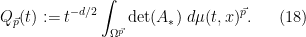
The determinant  is then a scalar element of the algebra (15). We then define the quantity
Example 8 Suppose we take  and let be natural numbers. Then can be viewed as the
  -matrix valued function

By slight abuse of notation, we write the determinant  of a matrix as
  , where and are the first and second rows of
  . Then


and after some calculation, one can then write  as
as


By a polynomial extrapolation argument, this formula is then also valid for fractional values of ; this can also be checked directly from the definitions after some tedious computation. Thus we see that while the compact-looking fractional dimensional integral (18) can be expressed in terms of more traditional integrals, the formulae get rather messy, even in the  case. As such, the fractional dimensional calculus (based heavily on derivative identities such as (16)) gives a more convenient framework to manipulate these otherwise quite complicated expressions.
Suppose the functions are close to constant matrices  , in the sense that
uniformly on for some small  (where we use for instance the operator norm to measure the size of matrices, and we allow implied constants in the
  notation to depend on
  , and the
  ). Then we can write
  for some bounded matrix
  , and then we can write
![\displaystyle A_* = \sum_{j=1}^k [A_j^0]_{1 \rightarrow p_j;j} + \varepsilon [B_j]_{1 \rightarrow p_j;j} = \sum_{j=1}^k p_j A_j^0 + \varepsilon \sum_{j=1}^k [B_j^0]_{1 \rightarrow p_j;j}.](https://s0.wp.com/latex.php?latex=%5Cdisplaystyle+A_%2A+%3D+%5Csum_%7Bj%3D1%7D%5Ek+%5BA_j%5E0%5D_%7B1+%5Crightarrow+p_j%3Bj%7D+%2B+%5Cvarepsilon+%5BB_j%5D_%7B1+%5Crightarrow+p_j%3Bj%7D+%3D+%5Csum_%7Bj%3D1%7D%5Ek+p_j+A_j%5E0+%2B+%5Cvarepsilon+%5Csum_%7Bj%3D1%7D%5Ek+%5BB_j%5E0%5D_%7B1+%5Crightarrow+p_j%3Bj%7D.&bg=ffffff&fg=000000&s=0&c=20201002)
We can therefore write

where  and the coefficients of the matrix
  are some polynomial combination of the coefficients of
 ![{[C_j^0]_{1 \rightarrow p_j;j}}](https://s0.wp.com/latex.php?latex=%7B%5BC_j%5E0%5D_%7B1+%5Crightarrow+p_j%3Bj%7D%7D&bg=ffffff&fg=000000&s=0&c=20201002) , with all coefficients in this polynomial of bounded size. As a consequence, and on expanding out all the fractional dimensional integrals, one obtains a formula of the form
, with all coefficients in this polynomial of bounded size. As a consequence, and on expanding out all the fractional dimensional integrals, one obtains a formula of the form

Thus, as long as  is strictly positive definite and
  is small enough, this quantity is comparable to the classical integral

Now we compute the time derivative of . We have

so by (16), one can write  as
as

![\displaystyle \mathrm{det}(A_*) \sum_{j=1}^k [\langle A_j(x-y_j),(x-y_j) \rangle]_{1 \rightarrow p_j;j}\ d\mu(t,x)^{\vec p}\ dx](https://s0.wp.com/latex.php?latex=%5Cdisplaystyle+%5Cmathrm%7Bdet%7D%28A_%2A%29+%5Csum_%7Bj%3D1%7D%5Ek+%5B%5Clangle+A_j%28x-y_j%29%2C%28x-y_j%29+%5Crangle%5D_%7B1+%5Crightarrow+p_j%3Bj%7D%5C+d%5Cmu%28t%2Cx%29%5E%7B%5Cvec+p%7D%5C+dx&bg=ffffff&fg=000000&s=0&c=20201002)
where we use  as the coordinate for the copy of that is being lifted to
  .
.
As before, we can take advantage of some cancellation in this expression using integration by parts. Since

where  are the standard basis for , we see from (16) and integration by parts that
![\displaystyle d Q_{\vec p}(t) = \frac{2\pi}{t^{\frac{d}{2}+1}} \int_{{\bf R}^d} \int_{\Omega^{\vec p}}\mathrm{det}(A_*) \sum_{j=1}^k x_i [\langle A_j(x-y_j), e_i\rangle]_{1 \rightarrow p_j;j}\ d\mu(t,x)^{\vec p}](https://s0.wp.com/latex.php?latex=%5Cdisplaystyle+d+Q_%7B%5Cvec+p%7D%28t%29+%3D+%5Cfrac%7B2%5Cpi%7D%7Bt%5E%7B%5Cfrac%7Bd%7D%7B2%7D%2B1%7D%7D+%5Cint_%7B%7B%5Cbf+R%7D%5Ed%7D+%5Cint_%7B%5COmega%5E%7B%5Cvec+p%7D%7D%5Cmathrm%7Bdet%7D%28A_%2A%29+%5Csum_%7Bj%3D1%7D%5Ek+x_i+%5B%5Clangle+A_j%28x-y_j%29%2C+e_i%5Crangle%5D_%7B1+%5Crightarrow+p_j%3Bj%7D%5C+d%5Cmu%28t%2Cx%29%5E%7B%5Cvec+p%7D&bg=ffffff&fg=000000&s=0&c=20201002)
with the usual summation conventions on the index  . Also, similarly to before, we suppose we have an element
  of (15) for each that does not depend on , then by (16) and integration by parts
![\displaystyle \int_{{\bf R}^d} \int_{\Omega^{\vec p}} \sum_{j=1}^k F_i [\langle A_j(x-y_j), e_i\rangle]_{1 \rightarrow p_j;j}\ d\mu(t,x)^{\vec p} = 0](https://s0.wp.com/latex.php?latex=%5Cdisplaystyle+%5Cint_%7B%7B%5Cbf+R%7D%5Ed%7D+%5Cint_%7B%5COmega%5E%7B%5Cvec+p%7D%7D+%5Csum_%7Bj%3D1%7D%5Ek+F_i+%5B%5Clangle+A_j%28x-y_j%29%2C+e_i%5Crangle%5D_%7B1+%5Crightarrow+p_j%3Bj%7D%5C+d%5Cmu%28t%2Cx%29%5E%7B%5Cvec+p%7D+%3D+0&bg=ffffff&fg=000000&s=0&c=20201002)
or, writing  ,
,
![\displaystyle \int_{{\bf R}^d} \int_{\Omega^{\vec p}} \sum_{j=1}^k \langle [A_j(x-y_j)]_{1 \rightarrow p_j;j}, F \rangle\ d\mu(t,x)^{\vec p} = 0.](https://s0.wp.com/latex.php?latex=%5Cdisplaystyle+%5Cint_%7B%7B%5Cbf+R%7D%5Ed%7D+%5Cint_%7B%5COmega%5E%7B%5Cvec+p%7D%7D+%5Csum_%7Bj%3D1%7D%5Ek+%5Clangle+%5BA_j%28x-y_j%29%5D_%7B1+%5Crightarrow+p_j%3Bj%7D%2C+F+%5Crangle%5C+d%5Cmu%28t%2Cx%29%5E%7B%5Cvec+p%7D+%3D+0.&bg=ffffff&fg=000000&s=0&c=20201002)
We can thus write (20) as

where  is the element of (15) given by
![\displaystyle G := \mathrm{det}(A_*) \sum_{j=1}^k [\langle A_j(x-y_j),(x-y_j) \rangle]_{1 \rightarrow p_j;j} \ \ \ \ \ (22)](https://s0.wp.com/latex.php?latex=%5Cdisplaystyle+G+%3A%3D+%5Cmathrm%7Bdet%7D%28A_%2A%29+%5Csum_%7Bj%3D1%7D%5Ek+%5B%5Clangle+A_j%28x-y_j%29%2C%28x-y_j%29+%5Crangle%5D_%7B1+%5Crightarrow+p_j%3Bj%7D+%5C+%5C+%5C+%5C+%5C+%2822%29&bg=ffffff&fg=000000&s=0&c=20201002)
![\displaystyle - \langle \sum_{j=1}^k [A_j(x-y_j)]_{1 \rightarrow p_j;j}, \mathrm{det}(A_*) x - F \rangle.](https://s0.wp.com/latex.php?latex=%5Cdisplaystyle+-+%5Clangle+%5Csum_%7Bj%3D1%7D%5Ek+%5BA_j%28x-y_j%29%5D_%7B1+%5Crightarrow+p_j%3Bj%7D%2C+%5Cmathrm%7Bdet%7D%28A_%2A%29+x+-+F+%5Crangle.&bg=ffffff&fg=000000&s=0&c=20201002)
The terms in  that are quadratic in cancel. The linear term can be rearranged as
![\displaystyle \langle x, A_* F - \mathrm{det}(A_*) \sum_{j=1}^k [A_j y_j]_{1 \rightarrow p_j; j} \rangle.](https://s0.wp.com/latex.php?latex=%5Cdisplaystyle+%5Clangle+x%2C+A_%2A+F+-+%5Cmathrm%7Bdet%7D%28A_%2A%29+%5Csum_%7Bj%3D1%7D%5Ek+%5BA_j+y_j%5D_%7B1+%5Crightarrow+p_j%3B+j%7D+%5Crangle.&bg=ffffff&fg=000000&s=0&c=20201002)
To cancel this, one would like to set equal to
![\displaystyle F = A_*^{-1}\mathrm{det}(A_*) \sum_{j=1}^k [A_j y_j]_{1 \rightarrow p_j; j} .](https://s0.wp.com/latex.php?latex=%5Cdisplaystyle+F+%3D+A_%2A%5E%7B-1%7D%5Cmathrm%7Bdet%7D%28A_%2A%29+%5Csum_%7Bj%3D1%7D%5Ek+%5BA_j+y_j%5D_%7B1+%5Crightarrow+p_j%3B+j%7D+.&bg=ffffff&fg=000000&s=0&c=20201002)
Now in the commutative algebra (15), the inverse  does not necessarily exist. However, because of the weight factor , one can work instead with the adjugate matrix
  , which is such that
  where
where  is the identity matrix. We therefore set equal to the expression
![\displaystyle F := \mathrm{adj}(A_*) \sum_{j=1}^k [A_j y_j]_{1 \rightarrow p_j; j}](https://s0.wp.com/latex.php?latex=%5Cdisplaystyle+F+%3A%3D+%5Cmathrm%7Badj%7D%28A_%2A%29+%5Csum_%7Bj%3D1%7D%5Ek+%5BA_j+y_j%5D_%7B1+%5Crightarrow+p_j%3B+j%7D&bg=ffffff&fg=000000&s=0&c=20201002)
and now the expression in (22) does not contain any linear or quadratic terms in . In particular it is completely independent of , and thus we can write
![\displaystyle G = \mathrm{det}(A_*) \sum_{j=1}^k [\langle A_j(\overline{y}-y_j),(\overline{y}-y_j) \rangle]_{1 \rightarrow p_j;j}](https://s0.wp.com/latex.php?latex=%5Cdisplaystyle+G+%3D+%5Cmathrm%7Bdet%7D%28A_%2A%29+%5Csum_%7Bj%3D1%7D%5Ek+%5B%5Clangle+A_j%28%5Coverline%7By%7D-y_j%29%2C%28%5Coverline%7By%7D-y_j%29+%5Crangle%5D_%7B1+%5Crightarrow+p_j%3Bj%7D&bg=ffffff&fg=000000&s=0&c=20201002)
![\displaystyle - \langle \sum_{j=1}^k [A_j(\overline{y}-y_j)]_{1 \rightarrow p_j;j}, \mathrm{det}(A_*) \overline{y} - F \rangle](https://s0.wp.com/latex.php?latex=%5Cdisplaystyle+-+%5Clangle+%5Csum_%7Bj%3D1%7D%5Ek+%5BA_j%28%5Coverline%7By%7D-y_j%29%5D_%7B1+%5Crightarrow+p_j%3Bj%7D%2C+%5Cmathrm%7Bdet%7D%28A_%2A%29+%5Coverline%7By%7D+-+F+%5Crangle&bg=ffffff&fg=000000&s=0&c=20201002)
where  is an arbitrary element of that we will select later to obtain a useful cancellation. We can rewrite this a little as
![\displaystyle G = \mathrm{det}(A_*) \sum_{j=1}^k [\langle A_j(\overline{y}-y_j),(\overline{y}-y_j) \rangle]_{1 \rightarrow p_j;j}](https://s0.wp.com/latex.php?latex=%5Cdisplaystyle+G+%3D+%5Cmathrm%7Bdet%7D%28A_%2A%29+%5Csum_%7Bj%3D1%7D%5Ek+%5B%5Clangle+A_j%28%5Coverline%7By%7D-y_j%29%2C%28%5Coverline%7By%7D-y_j%29+%5Crangle%5D_%7B1+%5Crightarrow+p_j%3Bj%7D+&bg=ffffff&fg=000000&s=0&c=20201002)
![\displaystyle - \langle \sum_{j=1}^k [A_j(\overline{y}-y_j)]_{1 \rightarrow p_j;j}, \mathrm{adj}(A_*) \sum_{j'=1}^k [A_j(\overline{y} - y_j)]_{1 \rightarrow p_j; j} \rangle.](https://s0.wp.com/latex.php?latex=%5Cdisplaystyle+-+%5Clangle+%5Csum_%7Bj%3D1%7D%5Ek+%5BA_j%28%5Coverline%7By%7D-y_j%29%5D_%7B1+%5Crightarrow+p_j%3Bj%7D%2C+%5Cmathrm%7Badj%7D%28A_%2A%29+%5Csum_%7Bj%27%3D1%7D%5Ek+%5BA_j%28%5Coverline%7By%7D+-+y_j%29%5D_%7B1+%5Crightarrow+p_j%3B+j%7D+%5Crangle.&bg=ffffff&fg=000000&s=0&c=20201002)
If we now introduce the matrix functions

and the vector functions

then this can be rewritten as
![\displaystyle G = \mathrm{det}(A_*) \sum_{j=1}^k [\|w_j\|^2]_{1 \rightarrow p_j;j}](https://s0.wp.com/latex.php?latex=%5Cdisplaystyle+G+%3D+%5Cmathrm%7Bdet%7D%28A_%2A%29+%5Csum_%7Bj%3D1%7D%5Ek+%5B%5C%7Cw_j%5C%7C%5E2%5D_%7B1+%5Crightarrow+p_j%3Bj%7D+&bg=ffffff&fg=000000&s=0&c=20201002)
![\displaystyle - \langle \sum_{j=1}^k [B_j w_j]_{1 \rightarrow p_j;j}, \mathrm{adj}(A_*) \sum_{j'=1}^k [B_j w_j]_{1 \rightarrow p_j; j} \rangle.](https://s0.wp.com/latex.php?latex=%5Cdisplaystyle+-+%5Clangle+%5Csum_%7Bj%3D1%7D%5Ek+%5BB_j+w_j%5D_%7B1+%5Crightarrow+p_j%3Bj%7D%2C+%5Cmathrm%7Badj%7D%28A_%2A%29+%5Csum_%7Bj%27%3D1%7D%5Ek+%5BB_j+w_j%5D_%7B1+%5Crightarrow+p_j%3B+j%7D+%5Crangle.&bg=ffffff&fg=000000&s=0&c=20201002)
Similarly to (19), suppose that we have

uniformly on , where  , thus we can write

for some bounded matrix-valued functions  . Inserting this into the previous expression (and expanding out appropriately) one can eventually write

where
![\displaystyle G^0 = \mathrm{det}(A^0_*) (\sum_{j=1}^k [\|w_j\|^2]_{1 \rightarrow p_j;j}](https://s0.wp.com/latex.php?latex=%5Cdisplaystyle+G%5E0+%3D+%5Cmathrm%7Bdet%7D%28A%5E0_%2A%29+%28%5Csum_%7Bj%3D1%7D%5Ek+%5B%5C%7Cw_j%5C%7C%5E2%5D_%7B1+%5Crightarrow+p_j%3Bj%7D&bg=ffffff&fg=000000&s=0&c=20201002)
![\displaystyle - \langle \sum_{j=1}^k B^0_j [w_j]_{1 \rightarrow p_j;j}, (A^0_*)^{-1} \sum_{j'=1}^k B^0_j [w_j]_{1 \rightarrow p_j; j} \rangle )](https://s0.wp.com/latex.php?latex=%5Cdisplaystyle+-+%5Clangle+%5Csum_%7Bj%3D1%7D%5Ek+B%5E0_j+%5Bw_j%5D_%7B1+%5Crightarrow+p_j%3Bj%7D%2C+%28A%5E0_%2A%29%5E%7B-1%7D+%5Csum_%7Bj%27%3D1%7D%5Ek+B%5E0_j+%5Bw_j%5D_%7B1+%5Crightarrow+p_j%3B+j%7D+%5Crangle+%29&bg=ffffff&fg=000000&s=0&c=20201002)
and  is some polynomial combination of the and
  (or more precisely, of the quantities
 ![{[D_j]_{1 \rightarrow p_j;j}}](https://s0.wp.com/latex.php?latex=%7B%5BD_j%5D_%7B1+%5Crightarrow+p_j%3Bj%7D%7D&bg=ffffff&fg=000000&s=0&c=20201002) ,
, ![{[w_j]_{1 \rightarrow p_j;j}}](https://s0.wp.com/latex.php?latex=%7B%5Bw_j%5D_%7B1+%5Crightarrow+p_j%3Bj%7D%7D&bg=ffffff&fg=000000&s=0&c=20201002) ,
, ![{[D_j w_j]_{1 \rightarrow p_j;j}}](https://s0.wp.com/latex.php?latex=%7B%5BD_j+w_j%5D_%7B1+%5Crightarrow+p_j%3Bj%7D%7D&bg=ffffff&fg=000000&s=0&c=20201002) ,
, ![{[\|w_j\|^2]_{1 \rightarrow p_j;j}}](https://s0.wp.com/latex.php?latex=%7B%5B%5C%7Cw_j%5C%7C%5E2%5D_%7B1+%5Crightarrow+p_j%3Bj%7D%7D&bg=ffffff&fg=000000&s=0&c=20201002) ) that is quadratic in the variables, with bounded coefficients. As a consequence, after expanding out the product fractional dimensional integrals and applying some Cauchy-Schwarz to control cross-terms, we have
) that is quadratic in the variables, with bounded coefficients. As a consequence, after expanding out the product fractional dimensional integrals and applying some Cauchy-Schwarz to control cross-terms, we have

![\displaystyle + O( \varepsilon t^{-\frac{d}{2}+2} \int_{{\bf R}^d} \int_{\Omega^{\vec p}} \sum_{j=1}^k [\| w_j \|^2]_{1 \rightarrow p_j;j}d\mu(t,x)^{\vec p}\ dx).](https://s0.wp.com/latex.php?latex=%5Cdisplaystyle+%2B+O%28+%5Cvarepsilon+t%5E%7B-%5Cfrac%7Bd%7D%7B2%7D%2B2%7D+%5Cint_%7B%7B%5Cbf+R%7D%5Ed%7D+%5Cint_%7B%5COmega%5E%7B%5Cvec+p%7D%7D+%5Csum_%7Bj%3D1%7D%5Ek+%5B%5C%7C+w_j+%5C%7C%5E2%5D_%7B1+%5Crightarrow+p_j%3Bj%7Dd%5Cmu%28t%2Cx%29%5E%7B%5Cvec+p%7D%5C+dx%29.&bg=ffffff&fg=000000&s=0&c=20201002)
Now we simplify  . We let

be the average value of  ; for each
  this is just a vector in . We then split
  , leading to the identities
![\displaystyle [\|w_j\|^2]_{1 \rightarrow p_j;j} = p_j \|\overline{w_j}\|^2 + 2 \langle \overline{w_j}, [w_j - \overline{w_j}]_{1 \rightarrow p_j;j}\rangle](https://s0.wp.com/latex.php?latex=%5Cdisplaystyle+%5B%5C%7Cw_j%5C%7C%5E2%5D_%7B1+%5Crightarrow+p_j%3Bj%7D+%3D+p_j+%5C%7C%5Coverline%7Bw_j%7D%5C%7C%5E2+%2B+2+%5Clangle+%5Coverline%7Bw_j%7D%2C+%5Bw_j+-+%5Coverline%7Bw_j%7D%5D_%7B1+%5Crightarrow+p_j%3Bj%7D%5Crangle+&bg=ffffff&fg=000000&s=0&c=20201002)
![\displaystyle + [\| w_j - \overline{w_j} \|^2]_{1 \rightarrow p_j;j}](https://s0.wp.com/latex.php?latex=%5Cdisplaystyle+%2B+%5B%5C%7C+w_j+-+%5Coverline%7Bw_j%7D+%5C%7C%5E2%5D_%7B1+%5Crightarrow+p_j%3Bj%7D&bg=ffffff&fg=000000&s=0&c=20201002)
and
![\displaystyle \sum_{j=1}^k B^0_j [w_j]_{1 \rightarrow p_j;j} = \sum_{j=1}^k p_j B^0_j \overline{w_j} + \sum_{j=1}^k B^0_j [(w_j - \overline{w_j})]_{1 \rightarrow p_j;j}.](https://s0.wp.com/latex.php?latex=%5Cdisplaystyle+%5Csum_%7Bj%3D1%7D%5Ek+B%5E0_j+%5Bw_j%5D_%7B1+%5Crightarrow+p_j%3Bj%7D+%3D+%5Csum_%7Bj%3D1%7D%5Ek+p_j+B%5E0_j+%5Coverline%7Bw_j%7D+%2B+%5Csum_%7Bj%3D1%7D%5Ek+B%5E0_j+%5B%28w_j+-+%5Coverline%7Bw_j%7D%29%5D_%7B1+%5Crightarrow+p_j%3Bj%7D.&bg=ffffff&fg=000000&s=0&c=20201002)
The term  is problematic, but we can eliminate it as follows. By construction one has (supressing the dependence on )
![\displaystyle \sum_{j=1}^k p_j B^0_j \overline{w_j} \int_{\Omega^p} \ d\mu^{\vec p} = \int_{\Omega^p} \sum_{j=1}^k B^0_j [w_j]_{1 \rightarrow p_j; j} \ d\mu^{\vec p}](https://s0.wp.com/latex.php?latex=%5Cdisplaystyle+%5Csum_%7Bj%3D1%7D%5Ek+p_j+B%5E0_j+%5Coverline%7Bw_j%7D+%5Cint_%7B%5COmega%5Ep%7D+%5C+d%5Cmu%5E%7B%5Cvec+p%7D+%3D+%5Cint_%7B%5COmega%5Ep%7D+%5Csum_%7Bj%3D1%7D%5Ek+B%5E0_j+%5Bw_j%5D_%7B1+%5Crightarrow+p_j%3B+j%7D+%5C+d%5Cmu%5E%7B%5Cvec+p%7D+&bg=ffffff&fg=000000&s=0&c=20201002)
![\displaystyle = \int_{\Omega^p}\sum_{j=1}^k B^0_j [B_j(\overline{y} - y_j)]_{1 \rightarrow p_j; j} \ d\mu^{\vec p}](https://s0.wp.com/latex.php?latex=%5Cdisplaystyle+%3D+%5Cint_%7B%5COmega%5Ep%7D%5Csum_%7Bj%3D1%7D%5Ek+B%5E0_j+%5BB_j%28%5Coverline%7By%7D+-+y_j%29%5D_%7B1+%5Crightarrow+p_j%3B+j%7D+%5C+d%5Cmu%5E%7B%5Cvec+p%7D&bg=ffffff&fg=000000&s=0&c=20201002)
![\displaystyle = \int_{\Omega^p}\sum_{j=1}^k B^0_j [B_j]_{1 \rightarrow p_j;j} \overline{y} - \int_{\Omega^p}\sum_{j=1}^k B^0_j [B_j y_j]_{1 \rightarrow p_j; j} \ d\mu^{\vec p}.](https://s0.wp.com/latex.php?latex=%5Cdisplaystyle+%3D+%5Cint_%7B%5COmega%5Ep%7D%5Csum_%7Bj%3D1%7D%5Ek+B%5E0_j+%5BB_j%5D_%7B1+%5Crightarrow+p_j%3Bj%7D+%5Coverline%7By%7D+-+%5Cint_%7B%5COmega%5Ep%7D%5Csum_%7Bj%3D1%7D%5Ek+B%5E0_j+%5BB_j+y_j%5D_%7B1+%5Crightarrow+p_j%3B+j%7D+%5C+d%5Cmu%5E%7B%5Cvec+p%7D.&bg=ffffff&fg=000000&s=0&c=20201002)
By construction, one has
![\displaystyle \int_{\Omega^p}\sum_{j=1}^k B^0_j [B_j]_{1 \rightarrow p_j;j}\ d\mu^{\vec p} = (\sum_{j=1}^k p B_0^j B_0^j + O(\varepsilon)) \int_{\Omega^p}\ d\mu^{\vec p}](https://s0.wp.com/latex.php?latex=%5Cdisplaystyle+%5Cint_%7B%5COmega%5Ep%7D%5Csum_%7Bj%3D1%7D%5Ek+B%5E0_j+%5BB_j%5D_%7B1+%5Crightarrow+p_j%3Bj%7D%5C+d%5Cmu%5E%7B%5Cvec+p%7D+%3D+%28%5Csum_%7Bj%3D1%7D%5Ek+p+B_0%5Ej+B_0%5Ej+%2B+O%28%5Cvarepsilon%29%29+%5Cint_%7B%5COmega%5Ep%7D%5C+d%5Cmu%5E%7B%5Cvec+p%7D+&bg=ffffff&fg=000000&s=0&c=20201002)

Thus if  is positive definite and is small enough, this matrix is invertible, and we can choose
  so that the expression
  vanishes. Making this choice, we then have
![\displaystyle \sum_{j=1}^k [B^0_j w_j]_{1 \rightarrow p_j;j} = \sum_{j=1}^k [B^0_j (w_j - \overline{w_j})]_{1 \rightarrow p_j;j}.](https://s0.wp.com/latex.php?latex=%5Cdisplaystyle+%5Csum_%7Bj%3D1%7D%5Ek+%5BB%5E0_j+w_j%5D_%7B1+%5Crightarrow+p_j%3Bj%7D+%3D+%5Csum_%7Bj%3D1%7D%5Ek+%5BB%5E0_j+%28w_j+-+%5Coverline%7Bw_j%7D%29%5D_%7B1+%5Crightarrow+p_j%3Bj%7D.&bg=ffffff&fg=000000&s=0&c=20201002)
Observe that the fractional dimensional integral of
![\displaystyle \langle \overline{w_j}, [w_j - \overline{w_j}]_{1 \rightarrow p_j;j} \rangle](https://s0.wp.com/latex.php?latex=%5Cdisplaystyle+%5Clangle+%5Coverline%7Bw_j%7D%2C+%5Bw_j+-+%5Coverline%7Bw_j%7D%5D_%7B1+%5Crightarrow+p_j%3Bj%7D+%5Crangle&bg=ffffff&fg=000000&s=0&c=20201002)
or
![\displaystyle \langle [w_j - \overline{w_j}]_{1 \rightarrow p_j;j}, M [w_{j'} - \overline{w_{j'}}]_{1 \rightarrow p_{j'};j'}](https://s0.wp.com/latex.php?latex=%5Cdisplaystyle+%5Clangle+%5Bw_j+-+%5Coverline%7Bw_j%7D%5D_%7B1+%5Crightarrow+p_j%3Bj%7D%2C+M+%5Bw_%7Bj%27%7D+-+%5Coverline%7Bw_%7Bj%27%7D%7D%5D_%7B1+%5Crightarrow+p_%7Bj%27%7D%3Bj%27%7D+&bg=ffffff&fg=000000&s=0&c=20201002)
for  and arbitrary constant matrices
  against
  vanishes. As a consequence, we can now simplify the integral

as

![\displaystyle + \langle [w_j - \overline{w_j}]_{1 \rightarrow p_j;j}, (1 - B_0^j (A^0_*)^{-1} B_0^{j}) [w_j - \overline{w_j}]_{1 \rightarrow p_j; j} \rangle\ d\mu^{\vec p}.](https://s0.wp.com/latex.php?latex=%5Cdisplaystyle+%2B+%5Clangle+%5Bw_j+-+%5Coverline%7Bw_j%7D%5D_%7B1+%5Crightarrow+p_j%3Bj%7D%2C+%281+-+B_0%5Ej+%28A%5E0_%2A%29%5E%7B-1%7D+B_0%5E%7Bj%7D%29+%5Bw_j+-+%5Coverline%7Bw_j%7D%5D_%7B1+%5Crightarrow+p_j%3B+j%7D+%5Crangle%5C+d%5Cmu%5E%7B%5Cvec+p%7D.&bg=ffffff&fg=000000&s=0&c=20201002)
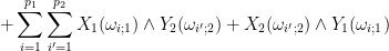
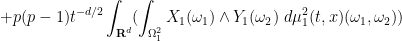
Using (2), we can split
![\displaystyle \langle [w_j - \overline{w_j}]_{1 \rightarrow p_j;j}, (1 - B_0^j (A^0_*)^{-1} B_0^{j}) [w_j - \overline{w_j}]_{1 \rightarrow p_j; j} \rangle](https://s0.wp.com/latex.php?latex=%5Cdisplaystyle+%5Clangle+%5Bw_j+-+%5Coverline%7Bw_j%7D%5D_%7B1+%5Crightarrow+p_j%3Bj%7D%2C+%281+-+B_0%5Ej+%28A%5E0_%2A%29%5E%7B-1%7D+B_0%5E%7Bj%7D%29+%5Bw_j+-+%5Coverline%7Bw_j%7D%5D_%7B1+%5Crightarrow+p_j%3B+j%7D+%5Crangle&bg=ffffff&fg=000000&s=0&c=20201002)
as the sum of
![\displaystyle [\langle w_j - \overline{w_j}, (1 - B_0^j (A^0_*)^{-1} B_0^{j}) (w_j - \overline{w_j}) \rangle ]_{1 \rightarrow p_j; j}](https://s0.wp.com/latex.php?latex=%5Cdisplaystyle+%5B%5Clangle+w_j+-+%5Coverline%7Bw_j%7D%2C+%281+-+B_0%5Ej+%28A%5E0_%2A%29%5E%7B-1%7D+B_0%5E%7Bj%7D%29+%28w_j+-+%5Coverline%7Bw_j%7D%29+%5Crangle+%5D_%7B1+%5Crightarrow+p_j%3B+j%7D&bg=ffffff&fg=000000&s=0&c=20201002)
and
![\displaystyle 2[\langle w_j(\omega_1) - \overline{w_j}, (1 - B_0^j (A^0_*)^{-1} B_0^{j}) (w_j(\omega_2) - \overline{w_j}) \rangle ]_{2 \rightarrow p_j; j}.](https://s0.wp.com/latex.php?latex=%5Cdisplaystyle+2%5B%5Clangle+w_j%28%5Comega_1%29+-+%5Coverline%7Bw_j%7D%2C+%281+-+B_0%5Ej+%28A%5E0_%2A%29%5E%7B-1%7D+B_0%5E%7Bj%7D%29+%28w_j%28%5Comega_2%29+-+%5Coverline%7Bw_j%7D%29+%5Crangle+%5D_%7B2+%5Crightarrow+p_j%3B+j%7D.&bg=ffffff&fg=000000&s=0&c=20201002)
The latter also integrates to zero by the mean zero nature of  . Thus we have simplified (24) to
![\displaystyle + [\langle w_j - \overline{w_j}, (1 - B_0^j (A^0_*)^{-1} B_0^{j}) (w_j - \overline{w_j}) \rangle ]_{1 \rightarrow p_j; j} \ d\mu^{\vec p}.](https://s0.wp.com/latex.php?latex=%5Cdisplaystyle+%2B+%5B%5Clangle+w_j+-+%5Coverline%7Bw_j%7D%2C+%281+-+B_0%5Ej+%28A%5E0_%2A%29%5E%7B-1%7D+B_0%5E%7Bj%7D%29+%28w_j+-+%5Coverline%7Bw_j%7D%29+%5Crangle+%5D_%7B1+%5Crightarrow+p_j%3B+j%7D+%5C+d%5Cmu%5E%7B%5Cvec+p%7D.&bg=ffffff&fg=000000&s=0&c=20201002)
Now let us make the key hypothesis that the matrix
is strictly positive definite, or equivalently that

for all  , where the ordering is in the sense of positive definite matrices. Then we have the pointwise bound

and thus

![\displaystyle \sum_{j=1}^k [\|\overline{w_j}\|^2 + \| w_j - \overline{w_j} \|^2 - O(\varepsilon) \|w_j\|^2 ]_{1 \rightarrow p_j;j}\ d\mu^{\vec p}\ dx.](https://s0.wp.com/latex.php?latex=%5Cdisplaystyle+%5Csum_%7Bj%3D1%7D%5Ek+%5B%5C%7C%5Coverline%7Bw_j%7D%5C%7C%5E2+%2B+%5C%7C+w_j+-+%5Coverline%7Bw_j%7D+%5C%7C%5E2+-+O%28%5Cvarepsilon%29+%5C%7Cw_j%5C%7C%5E2+%5D_%7B1+%5Crightarrow+p_j%3Bj%7D%5C+d%5Cmu%5E%7B%5Cvec+p%7D%5C+dx.&bg=ffffff&fg=000000&s=0&c=20201002)
For small enough, the expression inside the ![{[]_{1 \rightarrow p_j;j}}](https://s0.wp.com/latex.php?latex=%7B%5B%5D_%7B1+%5Crightarrow+p_j%3Bj%7D%7D&bg=ffffff&fg=000000&s=0&c=20201002) is non-negative, and we conclude the monotonicity
is non-negative, and we conclude the monotonicity

We have thus proven the following statement, which is essentially Proposition 4.1 of my paper with Bennett and Carbery:
Proposition 9 Let  , let
, let  be positive semi-definite real symmetric matrices, and let
  be such that

for  . Then for any positive measure spaces with measures
  and any functions
  on with
  for a sufficiently small , the quantity is non-decreasing in , and is also equal to
In particular, we have

for any .
A routine calculation shows that for reasonable choices of (e.g. discrete measures of finite support), one has

and hence (setting  ) we have

If we choose the to be the sum of  Dirac masses, and each to be the diagonal matrix
  , then the key condition (25) is obeyed for
  , and one arrives at the multilinear Kakeya inequality

whenever  are infinite tubes in of width
  and oriented within of the basis vector
  , for a sufficiently small absolute constant . (The hypothesis on the directions can then be relaxed to a transversality hypothesis by applying some linear transformations and the triangle inequality.)


21 comments
Comments feed for this article
29 June, 2019 at 8:42 pm
Anonymous
What are the main ideas? And what are you trying to achieve with the complex mathematics?
30 June, 2019 at 8:16 am
Anonymous
“One can wonder what the point is to all of this abstract formalism and how it relates to the rest of mathematics…” — Prof. Tao.
Some of us, I think, do not understand what you are doing here. Please explain to us in plain English, your goals and main ideas here. And maybe then, we can better appreciate the high-level mathematics associated with your ideas.
30 June, 2019 at 9:29 am
Anonymous
FYI: Please gather some information at the link below:
https://en.wikipedia.org/wiki/Kakeya_set
I hope it helps you.
1 July, 2019 at 11:46 am
Anonymous
Thanks! It helps a bit. That link is quite interesting! And I understand some of its content.
But ‘Symmetric functions in a fractional number of variables, and the multilinear Kakeya conjecture’ is generally beyond me, and it is probably meant for the elite few or insiders (highly specialized audience)…
C’est la vie.
26 July, 2019 at 6:42 pm
Anonymous
The ability to learn and the ability to absorb/understand complex or advanced mathematical ideas are a big part of any mathematician’s toolbox to solve problems or to do advanced research…
Please try solving some Diophantine equations (DEs) using two or more distinct variables (you may use parts of example 1 above as a starting point) to get some feel for the theory posted here.
And rethink (construct a counterexample or develop a different or simpler disproof or develop a general algorithm that solves DEs efficiently, etc.) the solution/disproof of David Hilbert’s Tenth Problem for inspiration and for purpose of learning/research. And good luck!
29 June, 2019 at 11:18 pm
Tony Carbery
Ron Blei did a lot of work on fractional cartesian products in the mid-1970’s to the mid 1980’s. Is there a connection with his work?
30 June, 2019 at 10:54 am
Terence Tao
Interesting (and I now remember that you actually had put this reference into our original paper and I had forgotten about it!). Looking at Blei’s work, it seems that he is focused on constructing fractal subsets of ambient Cartesian product spaces (such as ) which exhibit dimensional properties similar to that which one would expect a fractional Cartesian power to obey. The constructions here are more focused on the integration theory than the dimensional theory, but it could well be that when the exponent
  is a fraction
  then it is possible to find some more classical interpretation of these products, and of the fractional dimensional integral of symmetric functions, in a manner similar to what Blei does, and
29 June, 2019 at 11:44 pm
Allen Knutson
I haven’t done any calculations, but this is reminding me of Deligne’s tensor category of type A_n, n fractional. I’ll report back if it pans out.
29 June, 2019 at 11:52 pm
reader
What would we obtain if we were out for anti-symmetric functions in the first instance?
30 June, 2019 at 11:12 am
Terence Tao
Hmm, interesting question. From a representation theory perspective, symmetric functions correspond to Young diagrams consisting of one row, whereas antisymmetric functions correspond to Young diagrams consisting of one column. In this post we are focusing on trying to extend to situations where the horizontal dimensions of the Young diagram are fractional (perhaps related to this previous post: https://terrytao.wordpress.com/2017/09/05/continuous-analogues-of-the-schur-and-skew-schur-polynomials/ , now that I think about it) but if one were to try to do the same for antisymmetric functions then one would now also want to consider Young diagrams whose vertical dimensions are fractional. Perhaps this could be done, but it may require a somewhat different formalism than what is done here.
30 June, 2019 at 3:06 am
sylvainjulien
There must be a typo under your example 1, cause you define a quantity by setting it equal to itself.
[Corrected, thanks – T.]
30 June, 2019 at 8:29 am
L
@Allen_knutson Exactly what I was thinking. Etingoff’s work as well Representation theory in Complex dimension.
30 June, 2019 at 9:09 am
Anonymous
typo: The connection to ONE of these fractional dimensional integrals with more traditional integrals ultimately arises from the simple identity
[Reworded, thanks – T.]
30 June, 2019 at 11:21 pm
Anonymous
Is there a “natural” generalization of these concepts to the case of complex variables and complex valued functions?
Perhaps the concept of “symmetric function” should be replaced by a properly defined concept of “Hermitian complex valued function” ?
2 July, 2019 at 3:26 am
gpecc
The definition of![[F^{(k)}]_{k\rightarrow p}](https://s0.wp.com/latex.php?latex=%5BF%5E%7B%28k%29%7D%5D_%7Bk%5Crightarrow+p%7D&bg=ffffff&fg=545454&s=0&c=20201002) is what in Probability/Statistics is called a “symmetric U-statistic” with kernel
is what in Probability/Statistics is called a “symmetric U-statistic” with kernel  , based on a sample of dimension
  . U-statistics appear e.g. in parametric estimation, stochastic geometry, analysis of boolean functions, multiple stochastic integration, … It is intriguing to know that one can formally define symmetric U-statistics based on samples with fractional dimension…
2 July, 2019 at 9:00 am
Terence Tao
Thanks for this link to existing terminology! (Though it seems that the symmetric U-statistic actually corresponds to a normalised average that in my notation would be![\binom{p}{k}^{-1} [F^{(k)}]_{k \to p}](https://s0.wp.com/latex.php?latex=%5Cbinom%7Bp%7D%7Bk%7D%5E%7B-1%7D+%5BF%5E%7B%28k%29%7D%5D_%7Bk+%5Cto+p%7D&bg=ffffff&fg=545454&s=0&c=20201002) .)
.)
8 July, 2019 at 2:02 pm
p kothari
On random topic, what are your thoughts about What are your thoughts on analyzing Pauli–Lubanski pseudovector and spin number(information geometry) in NLP vectorized framework – doc2vec etc. to detect fake news?
8 July, 2019 at 5:17 pm
YY
How would he know?
29 July, 2019 at 10:30 am
Sharp bounds for multilinear curved Kakeya, restriction and oscillatory integral estimates away from the endpoint | What's new
[…] original proof of this proceeded using a heat flow monotonicity method, which in my previous post I reinterpreted using a “virtual integration” concept on a fractional Cartesian product […]
21 August, 2019 at 6:29 pm
tt
typo: The integrand on the left-hand side of (5) is![[x_1 x_2]_{2 \to p}](https://s0.wp.com/latex.php?latex=%5Bx_1+x_2%5D_%7B2+%5Cto+p%7D&bg=ffffff&fg=545454&s=0&c=20201002) .
.
[Corrected, thanks – T.]
15 April, 2020 at 8:04 pm
Lior Silberman
This is highly reminiscent of Razborov’s theory of flag algebras for extremal combinatorics.