You are currently browsing the tag archive for the ‘singular integrals’ tag.

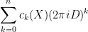
Kari Astala, Steffen Rohde, Eero Saksman and I have (finally!) uploaded to the arXiv our preprint “Homogenization of iterated singular integrals with applications to random quasiconformal maps“. This project started (and was largely completed) over a decade ago, but for various reasons it was not finalised until very recently. The motivation for this project was to study the behaviour of “random” quasiconformal maps. Recall that a (smooth) quasiconformal map is a homeomorphism {f: {\bf C} \rightarrow {\bf C}} that obeys the Beltrami equation

\displaystyle  \frac{\partial f}{\partial \overline{z}} = \mu \frac{\partial f}{\partial z}

for some Beltrami coefficient {\mu: {\bf C} \rightarrow D(0,1)}; this can be viewed as a deformation of the Cauchy-Riemann equation {\frac{\partial f}{\partial \overline{z}} = 0}. Assuming that {f(z)} is asymptotic to {z} 
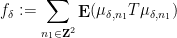
at infinity, one can (formally, at least) solve for {f} in terms of {\mu} 
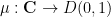
using the Beurling transform

\displaystyle  Tf(z) := \frac{\partial}{\partial z}(\frac{\partial f}{\partial \overline{z}})^{-1}(z) = -\frac{1}{\pi} p.v. \int_{\bf C} \frac{f(w)}{(w-z)^2}\ dw

by the Neumann series

\displaystyle  \frac{\partial f}{\partial \overline{z}} = \mu + \mu T \mu + \mu T \mu T \mu + \dots.

We looked at the question of the asymptotic behaviour of {f} if {\mu = \mu_\delta} is a random field that oscillates at some fine spatial scale {\delta>0}. A simple model to keep in mind is

\displaystyle  \mu_\delta(z) = \varphi(z) \sum_{n \in {\bf Z}^2} \epsilon_n 1_{n\delta + [0,\delta]^2}(z) \ \ \ \ \ (1)

where {\epsilon_n = \pm 1} are independent random signs and {\varphi: {\bf C} \rightarrow D(0,1)} 
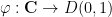
is a bump function. For models such as these, we show that a homogenisation occurs in the limit {\delta \rightarrow 0}
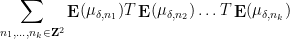
; each multilinear expression

\displaystyle  \mu_\delta T \mu_\delta \dots T \mu_\delta \ \ \ \ \ (2)

converges weakly in probability (and almost surely, if we restrict {\delta} to a lacunary sequence) to a deterministic limit, and the associated quasiconformal map {f = f_\delta} similarly converges weakly in probability (or almost surely). (Results of this latter type were also recently obtained by Ivrii and Markovic by a more geometric method which is simpler, but is applied to a narrower class of Beltrami coefficients.) In the specific case (1), the limiting quasiconformal map is just the identity map {f(z)=z}, but if for instance replaces the {\epsilon_n} by non-symmetric random variables then one can have significantly more complicated limits. The convergence theorem for multilinear expressions such as is not specific to the Beurling transform {T}; any other translation and dilation invariant singular integral can be used here.

The random expression (2) is somewhat reminiscent of a moment of a random matrix, and one can start computing it analogously. For instance, if one has a decomposition {\mu_\delta = \sum_{n \in {\bf Z}^2} \mu_{\delta,n}} such as (1), then (2) expands out as a sum

\displaystyle  \sum_{n_1,\dots,n_k \in {\bf Z}^2} \mu_{\delta,n_1} T \mu_{\delta,n_2} \dots T \mu_{\delta,n_k}

The random fluctuations of this sum can be treated by a routine second moment estimate, and the main task is to show that the expected value

\displaystyle  \sum_{n_1,\dots,n_k \in {\bf Z}^2} \mathop{\bf E}(\mu_{\delta,n_1} T \mu_{\delta,n_2} \dots T \mu_{\delta,n_k}) \ \ \ \ \ (3)

becomes asymptotically independent of {\delta}.

If all the {n_1,\dots,n_k} were distinct then one could use independence to factor the expectation to get

\displaystyle  \sum_{n_1,\dots,n_k \in {\bf Z}^2} \mathop{\bf E}(\mu_{\delta,n_1}) T \mathop{\bf E}(\mu_{\delta,n_2}) \dots T \mathop{\bf E}(\mu_{\delta,n_k})

which is a relatively straightforward expression to calculate (particularly in the model (1), where all the expectations here in fact vanish). The main difficulty is that there are a number of configurations in (3) in which various of the {n_j} collide with each other, preventing one from easily factoring the expression. A typical problematic contribution for instance would be a sum of the form

\displaystyle  \sum_{n_1,n_2 \in {\bf Z}^2: n_1 \neq n_2} \mathop{\bf E}(\mu_{\delta,n_1} T \mu_{\delta,n_2} T \mu_{\delta,n_1} T \mu_{\delta,n_2}). \ \ \ \ \ (4)

This is an example of what we call a non-split sum. This can be compared with the split sum

\displaystyle  \sum_{n_1,n_2 \in {\bf Z}^2: n_1 \neq n_2} \mathop{\bf E}(\mu_{\delta,n_1} T \mu_{\delta,n_1} T \mu_{\delta,n_2} T \mu_{\delta,n_2}). \ \ \ \ \ (5)

If we ignore the constraint {n_1 \neq n_2} in the latter sum, then it splits into

\displaystyle  f_\delta T g_\delta

where

\displaystyle  f_\delta := \sum_{n_1 \in {\bf Z}^2} \mathop{\bf E}(\mu_{\delta,n_1} T \mu_{\delta,n_1})

and

\displaystyle  g_\delta := \sum_{n_2 \in {\bf Z}^2} \mathop{\bf E}(\mu_{\delta,n_2} T \mu_{\delta,n_2})

and one can hope to treat this sum by an induction hypothesis. (To actually deal with constraints such as {n_1 \neq n_2} 
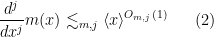
requires an inclusion-exclusion argument that creates some notational headaches but is ultimately manageable.) As the name suggests, the non-split configurations such as (4) cannot be factored in this fashion, and are the most difficult to handle. A direct computation using the triangle inequality (and a certain amount of combinatorics and induction) reveals that these sums are somewhat localised, in that dyadic portions such as

\displaystyle  \sum_{n_1,n_2 \in {\bf Z}^2: |n_1 - n_2| \sim R} \mathop{\bf E}(\mu_{\delta,n_1} T \mu_{\delta,n_2} T \mu_{\delta,n_1} T \mu_{\delta,n_2})

exhibit power decay in {R} 
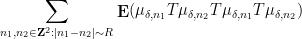
(when measured in suitable function space norms), basically because of the large number of times one has to transition back and forth between {n_1} and {n_2}. Thus, morally at least, the dominant contribution to a non-split sum such as (4) comes from the local portion when {n_2=n_1+O(1)}. From the translation and dilation invariance of {T} this type of expression then simplifies to something like

\displaystyle  \varphi(z)^4 \sum_{n \in {\bf Z}^2} \eta( \frac{n-z}{\delta} )

(plus negligible errors) for some reasonably decaying function {\eta}, and this can be shown to converge to a weak limit as {\delta \rightarrow 0}.

In principle all of these limits are computable, but the combinatorics is remarkably complicated, and while there is certainly some algebraic structure to the calculations, it does not seem to be easily describable in terms of an existing framework (e.g., that of free probability).

In contrast to previous notes, in this set of notes we shall focus exclusively on Fourier analysis in the one-dimensional setting {d=1} for simplicity of notation, although all of the results here have natural extensions to higher dimensions. Depending on the physical context, one can view the physical domain {{\bf R}} as representing either space or time; we will mostly think in terms of the former interpretation, even though the standard terminology of “time-frequency analysis”, which we will make more prominent use of in later notes, clearly originates from the latter.

In previous notes we have often performed various localisations in either physical space or Fourier space {{\bf R}}, for instance in order to take advantage of the uncertainty principle. One can formalise these operations in terms of the functional calculus of two basic operations on Schwartz functions {{\mathcal S}({\bf R})}, the position operator {X: {\mathcal S}({\bf R}) \rightarrow {\mathcal S}({\bf R})} defined by

\displaystyle  (Xf)(x) := x f(x)

and the momentum operator {D: {\mathcal S}({\bf R}) \rightarrow {\mathcal S}({\bf R})}, defined by

\displaystyle  (Df)(x) := \frac{1}{2\pi i} \frac{d}{dx} f(x). \ \ \ \ \ (1)

(The terminology comes from quantum mechanics, where it is customary to also insert a small constant {h} on the right-hand side of (1) in accordance with de Broglie’s law. Such a normalisation is also used in several branches of mathematics, most notably semiclassical analysis and microlocal analysis, where it becomes profitable to consider the semiclassical limit {h \rightarrow 0}, but we will not emphasise this perspective here.) The momentum operator can be viewed as the counterpart to the position operator, but in frequency space instead of physical space, since we have the standard identity

\displaystyle  \widehat{Df}(\xi) = \xi \hat f(\xi)

for any {\xi \in {\bf R}} and {f \in {\mathcal S}({\bf R})}. We observe that both operators {X,D} are formally self-adjoint in the sense that

\displaystyle  \langle Xf, g \rangle = \langle f, Xg \rangle; \quad \langle Df, g \rangle = \langle f, Dg \rangle

for all {f,g \in {\mathcal S}({\bf R})}, where we use the {L^2({\bf R})} Hermitian inner product

\displaystyle  \langle f, g\rangle := \int_{\bf R} f(x) \overline{g(x)}\ dx.

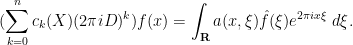
Clearly, for any polynomial {P(x)} of one real variable {x} (with complex coefficients), the operator {P(X): {\mathcal S}({\bf R}) \rightarrow {\mathcal S}({\bf R})} is given by the spatial multiplier operator

\displaystyle  (P(X) f)(x) = P(x) f(x)

and similarly the operator {P(D): {\mathcal S}({\bf R}) \rightarrow {\mathcal S}({\bf R})} is given by the Fourier multiplier operator

\displaystyle  \widehat{P(D) f}(\xi) = P(\xi) \hat f(\xi).

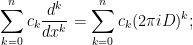
Inspired by this, if {m: {\bf R} \rightarrow {\bf C}} is any smooth function that obeys the derivative bounds

\displaystyle  \frac{d^j}{dx^j} m(x) \lesssim_{m,j} \langle x \rangle^{O_{m,j}(1)} \ \ \ \ \ (2)

for all {j \geq 0} and {x \in {\bf R}} (that is to say, all derivatives of {m} grow at most polynomially), then we can define the spatial multiplier operator {m(X): {\mathcal S}({\bf R}) \rightarrow {\mathcal S}({\bf R})} by the formula

\displaystyle  (m(X) f)(x) := m(x) f(x);

one can easily verify from several applications of the Leibniz rule that {m(X)} maps Schwartz functions to Schwartz functions. We refer to {m(x)} as the symbol of this spatial multiplier operator. In a similar fashion, we define the Fourier multiplier operator {m(D)} associated to the symbol {m(\xi)} by the formula

\displaystyle  \widehat{m(D) f}(\xi) := m(\xi) \hat f(\xi).

For instance, any constant coefficient linear differential operators {\sum_{k=0}^n c_k \frac{d^k}{dx^k}} can be written in this notation as

\displaystyle \sum_{k=0}^n c_k \frac{d^k}{dx^k} =\sum_{k=0}^n c_k (2\pi i D)^k;

however there are many Fourier multiplier operators that are not of this form, such as fractional derivative operators {\langle D \rangle^s = (1- \frac{1}{4\pi^2} \frac{d^2}{dx^2})^{s/2}} for non-integer values of {s}, which is a Fourier multiplier operator with symbol {\langle \xi \rangle^s}. It is also very common to use spatial cutoffs {\psi(X)} and Fourier cutoffs {\psi(D)} for various bump functions {\psi} to localise functions in either space or frequency; we have seen several examples of such cutoffs in action in previous notes (often in the higher dimensional setting {d>1}).

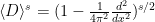
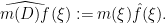
We observe that the maps {m \mapsto m(X)} and {m \mapsto m(D)} are ring homomorphisms, thus for instance

\displaystyle  (m_1 + m_2)(D) = m_1(D) + m_2(D)

and

\displaystyle  (m_1 m_2)(D) = m_1(D) m_2(D)

for any {m_1,m_2} obeying the derivative bounds (2); also {m(D)} is formally adjoint to {\overline{m(D)}} in the sense that

\displaystyle  \langle m(D) f, g \rangle = \langle f, \overline{m}(D) g \rangle

for {f,g \in {\mathcal S}({\bf R})}, and similarly for {m(X)} and {\overline{m}(X)}. One can interpret these facts as part of the functional calculus of the operators {X,D}, which can be interpreted as densely defined self-adjoint operators on {L^2({\bf R})}. However, in this set of notes we will not develop the spectral theory necessary in order to fully set out this functional calculus rigorously.

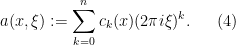
In the field of PDE and ODE, it is also very common to study variable coefficient linear differential operators
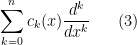
\displaystyle  \sum_{k=0}^n c_k(x) \frac{d^k}{dx^k} \ \ \ \ \ (3)

where the {c_0,\dots,c_n} are now functions of the spatial variable {x} obeying the derivative bounds (2). A simple example is the quantum harmonic oscillator Hamiltonian {-\frac{d^2}{dx^2} + x^2}. One can rewrite this operator in our notation as

\displaystyle  \sum_{k=0}^n c_k(X) (2\pi i D)^k

and so it is natural to interpret this operator as a combination {a(X,D)} of both the position operator {X} and the momentum operator {D}, where the symbol {a: {\bf R} \times {\bf R} \rightarrow {\bf C}} this operator is the function

\displaystyle  a(x,\xi) := \sum_{k=0}^n c_k(x) (2\pi i \xi)^k. \ \ \ \ \ (4)

Indeed, from the Fourier inversion formula
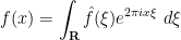
\displaystyle  f(x) = \int_{\bf R} \hat f(\xi) e^{2\pi i x \xi}\ d\xi

for any {f \in {\mathcal S}({\bf R})} we have

\displaystyle  (2\pi i D)^k f(x) = \int_{\bf R} (2\pi i \xi)^k \hat f(\xi) e^{2\pi i x \xi}\ d\xi

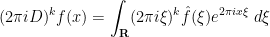
and hence on multiplying by {c_k(x)} and summing we have

\displaystyle (\sum_{k=0}^n c_k(X) (2\pi i D)^k) f(x) = \int_{\bf R} a(x,\xi) \hat f(\xi) e^{2\pi i x \xi}\ d\xi.

Inspired by this, we can introduce the Kohn-Nirenberg quantisation by defining the operator
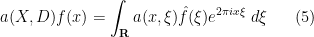
 {a(X,D) = a_{KN}(X,D): {\mathcal S}({\bf R}) \rightarrow {\mathcal S}({\bf R})} by the formula

\displaystyle  a(X,D) f(x) = \int_{\bf R} a(x,\xi) \hat f(\xi) e^{2\pi i x \xi}\ d\xi \ \ \ \ \ (5)

whenever {f \in {\mathcal S}({\bf R})} and {a: {\bf R} \times {\bf R} \rightarrow {\bf C}} is any smooth function obeying the derivative bounds

\displaystyle  \frac{\partial^j}{\partial x^j} \frac{\partial^l}{\partial \xi^l} a(x,\xi) \lesssim_{a,j,l} \langle x \rangle^{O_{a,j}(1)} \langle \xi \rangle^{O_{a,j,l}(1)} \ \ \ \ \ (6)

for all {j,l \geq 0} and {x \in {\bf R}} (note carefully that the exponent in {x} on the right-hand side is required to be uniform in {l}). This quantisation clearly generalises both the spatial multiplier operators {m(X)} and the Fourier multiplier operators {m(D)} defined earlier, which correspond to the cases when the symbol {a(x,\xi)} is a function of {x} only or {\xi} only respectively. Thus we have combined the physical space {{\bf R} = \{ x: x \in {\bf R}\}} and the frequency space {{\bf R} = \{ \xi: \xi \in {\bf R}\}} into a single domain, known as phase space {{\bf R} \times {\bf R} = \{ (x,\xi): x,\xi \in {\bf R} \}}. The term “time-frequency analysis” encompasses analysis based on decompositions and other manipulations of phase space, in much the same way that “Fourier analysis” encompasses analysis based on decompositions and other manipulations of frequency space. We remark that the Kohn-Nirenberg quantization is not the only choice of quantization one could use; see Remark 19 below.

Exercise 1

  • (i) Show that for {a} obeying (6), that {a(X,D)} does indeed map {{\mathcal S}({\bf R})} to {{\mathcal S}({\bf R})}.
  • (ii) Show that the symbol {a} is uniquely determined by the operator {a(X,D)}. That is to say, if {a,b} are two functions obeying (6) with {a(X,D) f = b(X,D) f} for all {f \in {\mathcal S}({\bf R})}, then {a=b}. (Hint: apply {a(X,D)-b(X,D)} to a suitable truncation of a plane wave {x \mapsto e^{2\pi i x \xi}} and then take limits.)

In principle, the quantisations {a(X,D)} are potentially very useful for such tasks as inverting variable coefficient linear operators, or to localize a function simultaneously in physical and Fourier space. However, a fundamental difficulty arises: map from symbols {a} to operators {a(X,D)} is now no longer a ring homomorphism, in particular

\displaystyle  (a_1 a_2)(X,D) \neq a_1(X,D) a_2(X,D) \ \ \ \ \ (7)

in general. Fundamentally, this is due to the fact that pointwise multiplication of symbols is a commutative operation, whereas the composition of operators such as {X} and {D} does not necessarily commute. This lack of commutativity can be measured by introducing the commutator

\displaystyle  [A,B] := AB - BA

of two operators {A,B}, and noting from the product rule that

\displaystyle  [X,D] = -\frac{1}{2\pi i} \neq 0.

(In the language of Lie groups and Lie algebras, this tells us that {X,D} are (up to complex constants) the standard Lie algebra generators of the Heisenberg group.) From a quantum mechanical perspective, this lack of commutativity is the root cause of the uncertainty principle that prevents one from simultaneously localizing in both position and momentum past a certain point. Here is one basic way of formalising this principle:

Exercise 2 (Heisenberg uncertainty principle) For any {x_0, \xi_0 \in {\bf R}} and {f \in \mathcal{S}({\bf R})}, show that

\displaystyle  \| (X-x_0) f \|_{L^2({\bf R})} \| (D-\xi_0) f\|_{L^2({\bf R})} \geq \frac{1}{4\pi} \|f\|_{L^2({\bf R})}^2.

(Hint: evaluate the expression {\langle [X-x_0, D - \xi_0] f, f \rangle} in two different ways and apply the Cauchy-Schwarz inequality.) Informally, this exercise asserts that the spatial uncertainty {\Delta x} and the frequency uncertainty {\Delta \xi} of a function obey the Heisenberg uncertainty relation {\Delta x \Delta \xi \gtrsim 1}.

Nevertheless, one still has the correspondence principle, which asserts that in certain regimes (which, with our choice of normalisations, corresponds to the high-frequency regime), quantum mechanics continues to behave like a commutative theory, and one can sometimes proceed as if the operators {X,D} (and the various operators {a(X,D)} constructed from them) commute up to “lower order” errors. This can be formalised using the pseudodifferential calculus, which we give below the fold, in which we restrict the symbol {a} to certain “symbol classes” of various orders (which then restricts {a(X,D)} to be pseudodifferential operators of various orders), and obtains approximate identities such as

\displaystyle  (a_1 a_2)(X,D) \approx a_1(X,D) a_2(X,D)

where the error between the left and right-hand sides is of “lower order” and can in fact enjoys a useful asymptotic expansion. As a first approximation to this calculus, one can think of functions {f \in {\mathcal S}({\bf R})} as having some sort of “phase space portrait{\tilde f(x,\xi)} which somehow combines the physical space representation {x \mapsto f(x)} with its Fourier representation {\xi \mapsto f(\xi)}, and pseudodifferential operators {a(X,D)} behave approximately like “phase space multiplier operators” in this representation in the sense that

\displaystyle  \widetilde{a(X,D) f}(x,\xi) \approx a(x,\xi) \tilde f(x,\xi).

Unfortunately the uncertainty principle (or the non-commutativity of {X} and {D}) prevents us from making these approximations perfectly precise, and it is not always clear how to even define a phase space portrait {\tilde f} of a function {f} precisely (although there are certain popular candidates for such a portrait, such as the FBI transform (also known as the Gabor transform in signal processing literature), or the Wigner quasiprobability distribution, each of which have some advantages and disadvantages). Nevertheless even if the concept of a phase space portrait is somewhat fuzzy, it is of great conceptual benefit both within mathematics and outside of it. For instance, the musical score one assigns a piece of music can be viewed as a phase space portrait of the sound waves generated by that music.

To complement the pseudodifferential calculus we have the basic Calderón-Vaillancourt theorem, which asserts that pseudodifferential operators of order zero are Calderón-Zygmund operators and thus bounded on {L^p({\bf R})} for {1 < p < \infty}. The standard proof of this theorem is a classic application of one of the basic techniques in harmonic analysis, namely the exploitation of almost orthogonality; the proof we will give here will achieve this through the elegant device of the Cotlar-Stein lemma.

Pseudodifferential operators (especially when generalised to higher dimensions {d \geq 1}) are a fundamental tool in the theory of linear PDE, as well as related fields such as semiclassical analysis, microlocal analysis, and geometric quantisation. There is an even wider class of operators that is also of interest, namely the Fourier integral operators, which roughly speaking not only approximately multiply the phase space portrait {\tilde f(x,\xi)} of a function by some multiplier {a(x,\xi)}, but also move the portrait around by a canonical transformation. However, the development of theory of these operators is beyond the scope of these notes; see for instance the texts of Hormander or Eskin.

This set of notes is only the briefest introduction to the theory of pseudodifferential operators. Many texts are available that cover the theory in more detail, for instance this text of Taylor.

Read the rest of this entry »

In the third of the Distinguished Lecture Series given by Eli Stein here at UCLA, Eli presented a slightly different topic, which is work in preparation with Alex Nagel, Fulvio Ricci, and Steve Wainger, on algebras of singular integral operators which are sensitive to multiple different geometries in a nilpotent Lie group.

Read the rest of this entry »

The first Distinguished Lecture Series at UCLA for this academic year is given by Elias Stein (who, incidentally, was my graduate student advisor), who is lecturing on “Singular Integrals and Several Complex Variables: Some New Perspectives“.  The first lecture was a historical (and non-technical) survey of modern harmonic analysis (which, amazingly, was compressed into half an hour), followed by an introduction as to how this theory is currently in the process of being adapted to handle the basic analytical issues in several complex variables, a topic which in many ways is still only now being developed.  The second and third lectures will focus on these issues in greater depth.

As usual, any errors here are due to my transcription and interpretation of the lecture.

[Update, Oct 27: The slides from the talk are now available here.]

Read the rest of this entry »

Archives