
You are currently browsing the tag archive for the ‘Poisson-Dirichlet process’ tag.
Define a partition of 

![{I \in (0,1]}](https://s0.wp.com/latex.php?latex=%7BI+%5Cin+%280%2C1%5D%7D&bg=ffffff&fg=000000&s=0&c=20201002)


- (Prime factorisation) Given a natural number
, one can decompose it into prime factors
(counting multiplicity), and then the multiset
is a partition of
- (Cycle decomposition) Given a permutation
on
, one can decompose
into cycles
, and then the multiset
is a partition of
- (Normalisation) Given a multiset
of positive real numbers whose sum
is finite and non-zero, the multiset
is a partition of
In the spirit of the universality phenomenon, one can ask what is the natural distribution for what a “typical” partition should look like; thus one seeks a natural probability distribution on the space of all partitions, analogous to (say) the gaussian distributions on the real line, or GUE distributions on point processes on the line, and so forth. It turns out that there is one natural such distribution which is related to all three examples above, known as the Poisson-Dirichlet distribution. To describe this distribution, we first have to deal with the problem that it is not immediately obvious how to cleanly parameterise the space of partitions, given that the cardinality of the partition can be finite or infinite, that multiplicity is allowed, and that we would like to identify two partitions that are permutations of each other
One way to proceed is to random partition 
![\displaystyle N_{[a,b]} := |\Sigma \cap [a,b]| = \sum_{x \in\Sigma} 1_{[a,b]}(x)](https://s0.wp.com/latex.php?latex=%5Cdisplaystyle+N_%7B%5Ba%2Cb%5D%7D+%3A%3D+%7C%5CSigma+%5Ccap+%5Ba%2Cb%5D%7C+%3D+%5Csum_%7Bx+%5Cin%5CSigma%7D+1_%7B%5Ba%2Cb%5D%7D%28x%29&bg=ffffff&fg=000000&s=0&c=20201002)
(where the cardinality here counts multiplicity). This can certainly be done, although in the case of the Poisson-Dirichlet process, the formulae for the joint distribution of such counting functions is moderately complicated. Another way to proceed is to order the elements of
with the convention that one pads the sequence 
![\displaystyle \{ (t_1,t_2,\ldots) \in [0,1]^{\bf N}: t_1 \geq t_2 \geq \ldots; \sum_{n=1}^\infty t_n = 1 \}.](https://s0.wp.com/latex.php?latex=%5Cdisplaystyle+%5C%7B+%28t_1%2Ct_2%2C%5Cldots%29+%5Cin+%5B0%2C1%5D%5E%7B%5Cbf+N%7D%3A+t_1+%5Cgeq+t_2+%5Cgeq+%5Cldots%3B+%5Csum_%7Bn%3D1%7D%5E%5Cinfty+t_n+%3D+1+%5C%7D.&bg=ffffff&fg=000000&s=0&c=20201002)
However, it turns out that the process of ordering the elements is not “smooth” (basically because functions such as 
It turns out that there is a better (or at least “smoother”) way to enumerate the elements 
- Given a partition
be an element of
having a probability
of being chosen as
occurs with multiplicity
, the net probability that
). Note that this is well-defined since the elements of
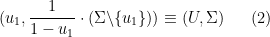
- Now suppose
is empty, we set
all equal to zero and stop. Otherwise, let
be an element of
chosen at random, with each element
having a probability
in
with probability
.)
- Now suppose
are both chosen. If
is empty, we set
all equal to zero and stop. Otherwise, let
be an element of
, with ech element
having a probability
- We continue this process indefinitely to create elements
.
We denote the random sequence ![{Enum(\Sigma) := (u_1,u_2,\ldots) \in [0,1]^{\bf N}}](https://s0.wp.com/latex.php?latex=%7BEnum%28%5CSigma%29+%3A%3D+%28u_1%2Cu_2%2C%5Cldots%29+%5Cin+%5B0%2C1%5D%5E%7B%5Cbf+N%7D%7D&bg=ffffff&fg=000000&s=0&c=20201002)
![{[0,1]^{\bf N}}](https://s0.wp.com/latex.php?latex=%7B%5B0%2C1%5D%5E%7B%5Cbf+N%7D%7D&bg=ffffff&fg=000000&s=0&c=20201002)

with 

Note that one can recover 

with the convention that one discards any zero elements on the right-hand side. Thus 
Note that this random enumeration procedure can also be adapted to the three models described earlier:
- Given a natural number
by letting each prime factor
of
with probability
, then once
be equal to
with probability
, and so forth.
- Given a permutation
, one can randomly enumerate its cycles
by letting each cycle
in
with probability
, and once
with probability
, and so forth. Alternatively, one traverse the elements of
- Given a multiset
is finite, we can randomly enumerate
the elements of this sequence by letting each
have a
probability of being set equal to
, and then once
have a
probability of being set equal to
, and so forth.
We then have the following result:
Proposition 1 (Existence of the Poisson-Dirichlet process) There exists a random partition
has the uniform distribution on
are independently and identically distributed copies of the uniform distribution on
.
A random partition

where 
An equivalent definition of a Poisson-Dirichlet process is a random partition
where 


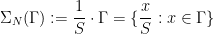
It turns out that each of the three ways to generate partitions listed above can lead to the Poisson-Dirichlet process, either directly or in a suitable limit. We begin with the third way, namely by normalising a Poisson process to have sum
Proposition 2 (Poisson-Dirichlet processes via Poisson processes) Let
, and let
be a Poisson process on
with intensity function
. Then the sum
is almost surely finite, and the normalisation
is a Poisson-Dirichlet process.
Again, we prove this proposition below the fold. Now we turn to the second way (a topic, incidentally, that was briefly touched upon in this previous blog post):
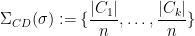
Proposition 3 (Large cycles of a typical permutation) For each natural number
. Then the random partition
converges in the limit
to a Poisson-Dirichlet process
in the following sense: given any fixed sequence of intervals
(independent of
converges in distribution to
.
Finally, we turn to the first way:
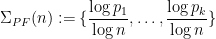
Proposition 4 (Large prime factors of a typical number) Let
, and let
be a random natural number chosen according to one of the following three rules:
- (Uniform distribution)
.
- (Shifted uniform distribution)
.
- (Zeta distribution) Each natural number
of being equal to
and
.
Then
converges as
to a Poisson-Dirichlet process
The process
The previous two propositions suggests an interesting analogy between large random integers and large random permutations; see this ICM article of Vershik and this non-technical article of Granville (which, incidentally, was once adapted into a play) for further discussion.
As a sample application, consider the problem of estimating the number 


![{[1/u,1]}](https://s0.wp.com/latex.php?latex=%7B%5B1%2Fu%2C1%5D%7D&bg=ffffff&fg=000000&s=0&c=20201002)


I thank Andrew Granville and Anatoly Vershik for showing me the nice link between prime factors and the Poisson-Dirichlet process. The material here is standard, and (like many of the other notes on this blog) was primarily written for my own benefit, but it may be of interest to some readers. In preparing this article I found this exposition by Kingman to be helpful.
Note: this article will emphasise the computations rather than rigour, and in particular will rely on informal use of infinitesimals to avoid dealing with stochastic calculus or other technicalities. We adopt the convention that we will neglect higher order terms in infinitesimal calculations, e.g. if 

Read the rest of this entry »

Recent Comments