
This week I am in Boston, giving this year’s Simons lectures at MIT together with David Donoho. (These lectures, incidentally, are endowed by Jim Simons, who was mentioned in some earlier discussion here.) While preparing these lectures, it occurred to me that I may as well post my lecture notes on this blog, since this medium is essentially just an asynchronous version of a traditional lecture series, and the hypertext capability is in some ways more convenient and informal than, say, 
I am giving three lectures, each expounding on some aspects of the theme “the dichotomy between structure and randomness”, which I also spoke about (and wrote about) for the ICM last August. This theme seems to pervade many of the areas of mathematics that I work in, and my lectures aim to explore how this theme manifests itself in several of these. In this, the first lecture, I describe the dichotomy as it appears in Fourier analysis and in number theory. (In the second, I discuss the dichotomy in ergodic theory and graph theory, while in the third, I discuss PDE.)
The “dichotomy between structure and randomness” seems to apply in circumstances in which one is considering a “high-dimensional” class of objects (e.g. sets of integers, functions on a space, dynamical systems, graphs, solutions to PDE, etc.). For sake of concreteness, let us focus today on sets of integers (later lectures will focus on other classes of objects). There are many different types of objects in these classes, however one can broadly classify them into three categories:
- Structured objects – objects with a high degree of predictability and algebraic structure. A typical example are the odd integers A = {…,-3,-1,1,3,5,…}. Note that if some large number n is known to lie in A, this reveals a lot of information about whether n+1, n+2, etc. will also lie in A. Structured objects are best studied using the tools of algebra and geometry.
- Pseudorandom objects – the opposite of structured; these are highly unpredictable and totally lack any algebraic structure. A good example is a randomly chosen set B of integers, in which each element n lies in B with an independent probability of 1/2. (One can imagine flipping a coin for each integer n, and defining B to be the set of n for which the coin flip resulted in heads.) Note that if some integer n is known to lie in B, this conveys no information whatsoever about the relationship of n+1, n+2, etc. with respect to B. Pseudorandom objects are best studied using the tools of analysis and probability.
- Hybrid sets – sets which exhibit some features of structure and some features of pseudorandomness. A good example is the primes P = {2,3,5,7,…}. The primes have some obvious structure in them: for instance, the prime numbers are all positive, they are all odd (with one exception), they are all adjacent to a multiple of six (with two exceptions), and their last digit is always 1, 3, 7, or 9 (with two exceptions). On the other hand, there is evidence that the primes, despite being a deterministic set, behave in a very “pseudorandom” or “uniformly distributed” manner. For instance, from the Siegel-Walfisz theorem we know that the last digit of large prime numbers is uniformly distributed in the set {1,3,7,9}; thus, if N is a large integer, the number of primes less than N ending in (say) 3, divided by the total number of primes less than N, is known to converge to 1/4 in the limit as N goes to infinity. In order to study hybrid objects, one needs a large variety of tools: one needs tools such as algebra and geometry to understand the structured component, one needs tools such as analysis and probability to understand the pseudorandom component, and one needs tools such as decompositions, algorithms, and evolution equations to separate the structure from the pseudorandomness. (More on this in later talks.)
A recurring question in many areas of analysis is the following: given a specific object (such as the prime numbers), can one determine precisely what the structured components are within the object, and how pseudorandom the remaining components of the object are? One reason for asking this question is that it often helps one compute various statistics (averages, sums, integrals, correlations, norms, etc.) of the object being studied. For instance, one can ask for how many twin pairs {n, n+2}, with n between 1 and N, one can find within a given set. In the structured set A given above, the answer is roughly N/2. For the random set B given above, the answer is roughly N/4; thus one sees that while A and B have exactly the same density (namely, 1/2), their statistics are rather different due to the fact that one is structured and one is random. As for the prime numbers, nobody knows what the answer is (though it is conjectured to be roughly 
The problem of determining exactly what the structured and pseudorandom components are of any given object is still largely intractable. However, what we have learnt in many cases is that we can at least show that an arbitrary object can be decomposed into some structured component and some pseudorandom component. Also there is often an orthogonality property (or dichotomy): if an object is orthogonal (or has small correlation with) all structured objects, then it is necessarily pseudorandom, and vice versa. Finally, we are sometimes lucky enough to be able to classify all the structured objects which are relevant for any given problem (e.g. computing a particular statistic). In such cases, one merely needs (in principle) to compute how the given object correlates with each member in one’s list of structured objects in order to determine what the desired statistic is. This is often simpler (though still non-trivial) than computing the statistic directly.
To illustrate these general principles, let us focus now on a specific area in analytic number theory, namely that of finding additive patterns in the prime numbers {2, 3, 5, 7, …}. Despite centuries of progress on these problems, many questions are still unsolved, for instance:
- Twin prime conjecture: There are infinitely many positive integers n such that n, n+2 are both prime.
- Sophie Germain prime conjecture: There are infinitely many positive integers n such that n, 2n+1 are both prime.
- Even Goldbach conjecture: For every even number
, there is a natural number n such that n, N-n are both prime.
On the other hand, we do have some positive results:
- Vinogradov’s theorem: For every sufficiently large odd number N, there are positive integers n, n’ such that n, n’, N-n-n’ are all prime. (The best explicit bound currently known for “sufficiently large” is
; the result has also been verified for
.)
- van der Corput’s theorem: There are infinitely many positive integers n, n’ such that n, n+n’, n+2n’ are all prime.
- Green-Tao theorem: For any positive integer k, there are infinitely many positive integers n, n’ such that n, n+n’, …, n+(k-1)n’ are all prime.
- A polynomial generalisation: For any integer-valued polynomials
with
, there are infinitely many positive integers n, n’ such that
are all prime.
As a general rule, it appears that it is feasible (after non-trivial effort) to find patterns in the primes involving two or more degrees of freedom (as described by the parameters n, n’ in above examples), but we still do not have the proper technology for finding patterns in the primes involving only one degree of freedom n. (This is of course an oversimplification; for instance, the pattern n, n+2, n’, n’+2 has two degrees of freedom, but finding infinitely many of these patterns in the primes is equivalent to the twin prime conjecture. If however one makes a non-degeneracy assumption, one can make the above claim more precise.)
One useful tool for establishing some (but not all) of the above positive results is Fourier analysis (which in this context is also known as the Hardy-Littlewood circle method). Rather than give the textbook presentation of that method here, let us try to motivate why Fourier analysis is an essential feature of many of these problems from the perspective of the dichotomy between structure and randomness, and in particular viewing structure as an obstruction to computing statistics which needs to be understood before the statistic can be accurately computed.
To treat many of the above questions concerning the primes in a unified manner, let us consider the following general setting. We consider k affine-linear forms 
- Question: does there there exist infinitely many r-tuples
of positive integers such that
are simulatenously prime?
For instance, the twin prime conjecture is the case when k=2, r=1, 


Because of the “obvious” structures in the primes, the answer to the above question can be “no”. For instance, since all but one of the primes are odd, we know that there are not infinitely many patterns of the form n, n+1 in the primes, because it is not possible for n, n+1 to both be odd. More generally, given any prime q, we know that all but one of the primes is coprime to q. Hence, if it is not possible for
Another obstruction comes from the trivial observation that the primes are all positive. Hence, if it is not possible for 
It is conjectured that these “local” obstructions are the only obstructions to solvability of the above question. More precisely, we have
- Dickson’s conjecture: If there are no obstructions at any prime q, and there are no obstructions at infinity, then the answer to the above question is “yes”.
This conjecture would imply the twin prime and Sophie Germain conjectures, as well as the Green-Tao theorem; it also implies the Hardy-Littlewood prime tuples conjecture as a special case. There is a quantitative version of this conjecture which predicts a more precise count as to how many solutions there are in a given range, and which would then also imply Vinogradov’s theorem, as well as Goldbach’s conjecture (for sufficiently large N); see this paper for further discussion. As one can imagine, this conjecture is still largely unsolved, however there are many important special cases that have now been established – several of which via the Hardy-Littlewood circle method.
One can view Dickson’s conjecture as an impossibility statement: that it is impossible to find any other obstructions to solvability for linear patterns in the primes than the obvious local obstructions at primes q and at infinity. (It is also a good example of a local-to-global principle, that local solvability implies global solvability.) Impossibility statements have always been very difficult to prove – one has to locate all possible obstructions to solvability, and eliminate each one of them in turn. In particular, one has to exclude various exotic “conspiracies” between the primes to behave in an unusually structured manner that somehow manages to always avoid all the patterns that one is seeking within the primes. How can one disprove a conspiracy?
To give an example of what such a “conspiracy” might look like, consider the twin prime conjecture, that of finding infinitely many pairs n, n+2 which are both prime. This pattern encounters no obstructions at primes q or at infinity and so Dickson’s conjecture predicts that there should be infinitely many such patterns. In particular, there are no obstructions at 3 because prime numbers can equal 1 or 2 mod 3, and it is possible to find pairs n, n+2 which also have this property. But suppose that it transpired that all but finitely many of the primes ended up being 2 mod 3. From looking at tables of primes this seems to be unlikely, but it is not immediately obvious how to disprove it; it could well be that once one reaches, say, 
To look for other conspiracies that one needs to eliminate, let us rewrite the conspiracy “all but finitely many of the primes are 2 mod 3” in the more convoluted format

where {x} is the fractional part of x. This type of conspiracy can now be generalised, for instance consider the statement

Again, such a conspiracy seems very unlikely – one would expect these fractional parts to be uniformly distributed between 0 and 1, rather than concentrate all in the interval [0, 0.01] – but it is hard to rule this conspiracy out a priori. And if this conspiracy (*) was in fact true, then the twin prime conjecture would be false, as can be quickly seen by considering the identity

which forbids the two fractional parts on the left-hand side to simultaneously fall in the interval [0, 0.01]. Thus, in order to solve the twin prime conjecture, one must rule out (*). Fortunately, it has been known since the work of Vinogradov that 


and we now see the appearance of Fourier analysis in this subject.
One can rather easily concoct an endless stream of further conspiracies, each of which could contradict the twin prime conjecture; this is one of the reasons why this conjecture is considered so difficult. Let us thus leave this conjecture for now and consider some two-parameter problems. Consider for instance the problem of finding infinitely many patterns of the form n, n+n’, n+2n’+2 (i.e. arithmetic progressions of length 3, but with the last element shifted by 2). Once again, the conspiracy (*), if true, would obstruct solvability for this pattern, due to the easily verified identity

which is related to the fact that the function 
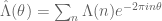
More generally, we can see that if the primes correlate in some unusual way with a linear character 


for all positive integers n; this identity is a restatement of the fundamental theorem of arithmetic, and in fact defines the von Mangoldt function uniquely. The problem of counting patterns {n, n+n’, n+2n’+2} is then roughly equivalent to the task of computing sums such as

where we shall be intentionally vague as to what range the variables n, n’ will be summed over. We have the Fourier inversion formula

where
is a sum very similar in nature to the sums 

Thus, if one gets good enough control on the Fourier coefficients 

I have glossed over the question of how one actually computes the Fourier coefficients

where 

and then one uses the irrationality of 

Now suppose we look at progressions of length 4: n, n+n’, n+2n’, n+3n’. As with progressions of length 3, “linear” or “Fourier” conspiracies such as (*) will bias or distort the total count of such progressions in the primes less than a given number N. But, in contrast to the length 3 case where these are the only conspiracies that actually influence things, for length 4 progressions there are now “quadratic” conspiracies which can cause trouble. Consider for instance the conspiracy
This conspiracy, which can exist even when all linear conspiracies are eliminated, will significantly bias the number of progressions of length 4, due to the identity


which is related to the fact that the function 

![0 < \{ [\sqrt{2} p] \sqrt{3} p \} < 0.01](https://s0.wp.com/latex.php?latex=0+%3C+%5C%7B+%5B%5Csqrt%7B2%7D+p%5D+%5Csqrt%7B3%7D+p+%5C%7D+%3C+0.01&bg=ffffff&fg=545454&s=0&c=20201002)
where [] is the greatest integer function. The point here is that the function ![{}[\sqrt{2} x] \sqrt{3} x](https://s0.wp.com/latex.php?latex=%7B%7D%5B%5Csqrt%7B2%7D+x%5D+%5Csqrt%7B3%7D+x&bg=ffffff&fg=545454&s=0&c=20201002)

![\sum_{p < N} e^{2\pi i [\sqrt{2} p] \sqrt{3} p}](https://s0.wp.com/latex.php?latex=%5Csum_%7Bp+%3C+N%7D+e%5E%7B2%5Cpi+i+%5B%5Csqrt%7B2%7D+p%5D+%5Csqrt%7B3%7D+p%7D&bg=ffffff&fg=545454&s=0&c=20201002)

The method also works for other linear patterns of comparable “complexity” to progressions of length 4. We are currently working on the problem of longer progressions, in which cubic and higher order obstructions appear (which should be modeled by 3-step and higher nilsequences); some work related to this should appear here shortly.

44 comments
Comments feed for this article
6 April, 2007 at 5:48 pm
stevenm
Hi Terry,
Your chosen theme “dichotomy between structure and randomness” is certainly a very interesting one not only in mathematics but in theoretical physics, complexity and biology: fluctuations or randomness will give
rise to the growth of structure, whether it is galaxies arising from
randomness in the early universe, or the complexity and the evolution of biological structures. The effect of random noise on multi-dimensional nonlinear systems is also of much interest, for example in turbulence or pattern formation. As regards the pseudorandom objects you mention, an open problem should surely still be whether one can truly distinguish
between a pseudorandom sequence and a truly random sequence, without knowing the generating algorithm that was used and the state in which it was initially prepared. The security of most encryption algorithms I assume would be based on the assumption that it is actually totally impossible to distinguish between these. (Is it though?). Von Neumann remarked that those who think they can generate random numbers using arithmetical algorithms are “in sin”. But since his time some rather sophisticated pseudorandom number generators have evolved such as the ‘Blum Blum Shub’, the ‘Fortuna’ and the ‘Mersenne Twister’. Could the output of one of these be distinguished–within a tractable sample size–from a truly random number sequence that has been generated via a physical process such as thermal noise or a quantum process like radioactive decay? Monte Carlo simulations in physics and finance etc. will assume that a pseudo-random sequence is good enough for the simulation of processes that are expected to be truly random. I was also curious whether your interests have ever included, or currently include, stochastic partial differential equations (SPDEs) or “stochastic geometries”; geometries or geometric structures that fluctuate or evolve in a random way?
7 April, 2007 at 8:51 am
Terence Tao
Dear Stevenm,
There is certainly an analogy between algorithmic pseudorandomness, and the type of pseudorandomness that I will talk about in these lectures (Fourier pseudorandomness (Gowers uniformity), ergodic pseudorandomness (mixing), graph pseudorandomness (regularity), and dispersive pseudorandomness (local decay). For instance, if one views an algorithm as a finite state machine, then the running of this algorithm does resemble a kind of discrete version of a dynamical system. I am not an expert in computational complexity, but it appears though that the analogous questions for algorithmic pseudorandomness are significantly more difficult to answer, touching on major unsolved problems such as and
and  .
.
There is a heuristic conjecture that the primes (or more precisely, the Möbius function ) are so “algorithmically pseudorandom” that they having vanishing asymptotic correlation with any “finite complexity” bounded sequence a(n), though I am not sure I can define what “finite complexity” means precisely (something like the output at time n of a dynamical system which can be described algebraically using only finitely many symbols). This conjecture, even if it is stated rigorously, is probably beyond the reach of current technology.
Incidentally, I do have a project on random quasiconformal geometries, which should appear here in a few months.
7 April, 2007 at 9:01 am
Simons Lecture II: Structure and randomness in ergodic theory and graph theory « What’s new
[…] the last lecture we saw that sets of integers could be divided (rather informally) into structured sets, […]
7 April, 2007 at 10:11 am
Greg Kuperberg
The conjecture that is much more to the point of algorithmic pseudorandomness than
  . There is a theorem that
  relative to a random oracle, i.e., that
  if
if  is a randomly chosen Boolean function. The exponential notation means that that
  is supplied to the computer as a black-box function. The proof is the classic, original derandomization argument. If you run the randomized algorithm with the pseudorandom source with enough trials, and then combine the results with majority rule, then consensus will be wrong for only finitely many inputs with probability 1, with respect to the random choice of
  . An algorithm that is only wrong for finitely many inputs can be repaired to one that is always right.
Much of the work in showing that has gone into replacing
  with a cryptographic function
  . If you imagine using
  is the above derandomization argument, then the requirement on
  is exactly that it should be cryptographically pseudorandom. Because, you can pick the algorithm to be anything that attempts to distinguish
  from a truly random
  . (Note the two uses of the word “random” here.
  means algorithms that are allowed randomness on the fly, whlie
  is deterministic algorithms with a randomly chosen, infinite ROM table.)
Essentially, people believe that because they believe that universal pseudorandom functions
  exist. In fact, they can make specific examples, they just can’t prove that they work. I have the feeling that there are weaker circumstances that still prove that
  , but this is a summary of what people think is really going on.
7 April, 2007 at 10:51 pm
Emmanuel Kowalski
Concerning exponential sums over primes, I wonder what you might think about exponential sums involving sqrt(p), in particular what kind of “conspiracies” or
natural problems they could be related to?
The point is that Iwaniec, Luo and Sarnak have related such exponential sums
to the Riemann Hypothesis for certain modular L-functions (see
http://www.numdam.org/numdam-bin/fitem?id=PMIHES_2000__91__55_0
specifically their Hypothesis (S), discussed in Section 10, and Appendix C;
technically, good cancellation in sums with sqrt(p) uniformly over arithmetic
progressions would lead to a zero-free strip, under some condition).
There is definitely a group underlying their work, namely SL(2,Z).
8 April, 2007 at 9:23 am
Terence Tao
Dear Emmanuel,
Thank you very much for your comment! I had heard of the ILS paper before but had not had a chance to seriously look at it.
There are two sorts of conspiracies: blatant conspiracies, which for instance prevent for various “algebraic” functions
  , and the much weaker spoiler conspiracies, which instead cause just enough non-randomness to prevent
  . A single zero of an L-function off the critical line, for instance, is a spoiler conspiracy, whereas one at 1 or at 1+it is a blatant conspiracy. I don’t really have the courage to state what spoiler conspiracies are possible – and the Hypothesis S in ILS is of a “no spoiler conspiracy” type. But it seems plausible that the only blatant conspiracies that the primes have are the “obvious” ones, coming from local considerations.
The story may be more complicated if one restricts to a thinner set than the full integers or the full primes, such as polynomial sequences f(T), where T ranges over the integers. For instance, in the “finite field model” in which the integers are replaced by a polynomial ring![k[u]](https://s0.wp.com/latex.php?latex=k%5Bu%5D&bg=ffffff&fg=545454&s=0&c=20201002) over a finite field, Conrad-Conrad-Gross have a blatant conspiracy that shows that certain one-variable polynomials f(T) are biased to not be prime despite avoiding all obvious local obstructions (e.g. reducibility) – though this particular conspiracy is very much a feature of the finite characteristic of the underlying field. Then of course there are all the Hilbert 10th problem constructions, such as polynomials whose positive values are precisely the primes, and so forth. So I would be hesitant to make any grand conjectures on sparse sets, such as those given by polynomials or group actions, at present (though I hear that Bourgain, Gamburd, and Sarnak have made some very recent advances in this direction, at least regarding almost primes instead of primes).
over a finite field, Conrad-Conrad-Gross have a blatant conspiracy that shows that certain one-variable polynomials f(T) are biased to not be prime despite avoiding all obvious local obstructions (e.g. reducibility) – though this particular conspiracy is very much a feature of the finite characteristic of the underlying field. Then of course there are all the Hilbert 10th problem constructions, such as polynomials whose positive values are precisely the primes, and so forth. So I would be hesitant to make any grand conjectures on sparse sets, such as those given by polynomials or group actions, at present (though I hear that Bourgain, Gamburd, and Sarnak have made some very recent advances in this direction, at least regarding almost primes instead of primes).
8 April, 2007 at 5:00 pm
Paul Krapivsky
Sorry, this is the last try…
Dear Terry and Emmanuel,
Another potentially interesting problem is the distribution of gaps in the sequence of fractional part of square-roots of primes. If one considers the sequence {n^a}, with some 0
8 April, 2007 at 8:41 pm
Terence Tao
Dear Paul,
I think your comments are turning the < signs into HTML. You can try using < and > instead. I know, it’s a pain, I wish I could do something about it…
9 April, 2007 at 3:56 am
Emmanuel Kowalski
I definitely agree with the distinction between “spoiler” and “blatant” conspiracies.
In classical prime number theory, it seems that most “blatant” conspiracies
are really symptoms of ignorance: they can/should be incorporated to the “main
term” (but of course that can be wishful thinking…), or used to reformulate the original
problem (e.g. p-1 can not be prime infinitely often, but (p-1)/2 can…).
Another (maybe) interesting point is that when we deal with prime numbers, sometimes
difficulties are really inherited from the integers. This is very clear when using sieve methods; for instance, in the type of problems that Bourgain, Sarnak and Gamburd are investigating (looking at points with prime or almost prime coordinates in orbits of certain groups actions, etc) even the corresponding counting problem for integers are hard, but they more or less have to be used as a starting point for looking at primes with sieve.
On the other hand, their problems, as far as I understand, do not actually involve sums
over primes (or integers) with functions like sqrt(p) — and correspondingly, the source
of cancellation lies in spectral gaps of various types (Selberg’s theorem, approximations to Ramanujan-Petersson conjecture, and especially expanding graphs in the more combinatorial settings, etc).
9 April, 2007 at 10:08 am
Paul Krapivsky
Dear Terry and Emmanuel,
Another potentially interesting problem is the distribution of gaps in the sequence of fractional part of square-roots of primes. If one considers the sequence {n^A} of natural numbers n=1,…,N, and multiplies the gap lengths by N, the gap distribution becomes exponential in the large N limit for all exponents A (between 0 and 1) except A=1/2. This is an astonishing experimental observation; for A=1/2 the gap length distribution was recently found by Elskies and McMullen, and it is indeed very different from exponential — it exhibits two `phase transitions’ and it has an algebraic tail. It is possible of course that the replacement of the whole numbers by primes merely makes the problem difficult but does not alter the gap distribution.
10 April, 2007 at 10:19 am
Not Even Wrong » Blog Archive » Math and Physics Roundup
[…] of the highest possible quality, see Terry Tao’s postings on his Simons lectures at MIT, here, here and […]
14 April, 2007 at 6:31 pm
Terence Tao
Dear Paul,
Gap distributions in any statistics related to primes are of course very interesting, but also well beyond our current technology; they seem to require knowing an incredible amount of “fine-scale” or “local” behaviour for the primes, whereas our current analytic knowledge primarily extends to rather “coarse-scale” or “aggregate” statistics; even the generalised Riemann hypothesis, while it would dramatically improve our coarse-scale control of the primes, doesn’t actually do much for the fine-scale questions (e.g. the twin prime conjecture doesn’t seem to become much easier on GRH). Even finding the right conjectures to make for, say, the asymptotic distribution of prime gaps , is remarkably subtle. Perhaps the best way to proceed here is simply by numerics, to see if anything unexpected happens – I would guess that the gap distribution for {p^A} would be similar to {n^A}, especially near generic (e.g. Diophantine) points in [0,1], but it could well be that some unusual irregularity emerges.
17 April, 2007 at 4:06 pm
As coisinhas interessantes de hoje… at It’s Equal but It’s Different
[…] Simons Lecture I: Structure and randomness in Fourier analysis and number theory; […]
27 April, 2007 at 10:43 am
Fields Medalist Symposium « What’s new
[…] I gave a more detailed presentation of the material I had discussed in my first Simons lecture, and focussing a bit more on the role of nilflows in characterising the “structure” or […]
2 May, 2007 at 7:06 am
Distinguished Lecture Series I: Shou-wu Zhang, "Overview of rational points on curves" « What’s new
[…] the to be non-zero (otherwise there is a local obstruction at p, similar to what I discussed in my first Simons lecture). Hasse formed his famous local-to-global principle, which is the heuristic that the converse […]
18 May, 2007 at 4:47 pm
warren smith
I want to know the following.
Are there an infinite number of 2-tuples (p,q) of odd primes such that
(p-1)*(q-1) is a product of at most a constant number of primes.
And is this still true if we demand both p and q be larger than C
(for any particular C)?
It sounds like this is similar to things you and Chen Jing-Run could do…
18 May, 2007 at 8:19 pm
Terence Tao
Dear Warren,
The argument of Chen will give infinitely many primes p for which (p-1)/2 is the product of at most 2 primes, which then in turn gives arbitrarily large pairs (p-1)(q-1) which is the product of at most 4 primes, times 4 (so six primes in all). This is probably the best one can do with current technology, due to the parity problem (I plan to post more on this in the future).
One does not quite need the full power of Chen’s result to get a qualitative result of this nature; using slightly lower-tech methods such as the Selberg sieve coupled with the Bombieri-Vinogradov inequality, one can achieve the same result but with O(1) primes in the prime factorisation of (p-1)(q-1).
19 May, 2007 at 2:30 pm
warren smith
to TT: I sent you some email, it appears your precediing post is the extra ingredient I needed to solve an open problem in coding theory.
(Or I’m just wrong.) Anyway, read the email. Cheerio.
25 May, 2007 at 7:48 pm
Primes in Pre-K « Home Schooled
[…] primes. See, pattern!” For a second I thought he’d been to one of Terry Tao’s lectures… The number 33 sort of burst his bubble. Still, he keeps […]
31 July, 2007 at 4:51 pm
Structure and randomness in combinatorics « What’s new
[…] 2007 conference in October. This tutorial covers similar ground as my ICM paper (or slides), or my first two Simons lectures, but focuses more on the “nuts-and-bolts” of how structure theorems […]
14 August, 2007 at 9:58 pm
Martin Winer
Hi Terry,
I don’t claim to be in your league in mathematics, just the same, you never know. Sometimes an amature’s view of the problem can help the pro’s figure things out. In my mind randomness is determinism cross recursive self complication. I use this idea to probe primes using a recursively self complicating algorithm Pat(f(n)) which lays down the primes.
The quick explanation is here:
http://www.rankyouragent.com/primes/primes_simple.htm
The more detailed version is here:
http://www.rankyouragent.com/primes/primes.htm
Best regards and good luck in your search…MCW
1 September, 2007 at 6:42 am
Anonymous
you are good on elementry prime number methods but do not discuss the langlands conjecture
9 October, 2007 at 2:41 am
Mario
It is always interesting to consider the subject of generating random
numbers – but – given that ‘EVERYTHING’ around us in the physical
sense is ‘computing’ and given that ALL ‘computations are at least
‘POTENTIALLY’ reversible (if you could live long enough…what exactly
is ‘RANDOM’?
9 October, 2007 at 8:47 am
Terence Tao
Dear Mario,
It may well be that the universe itself is completely deterministic (though this depends on what the “true” laws of physics are, and also to some extent on certain ontological assumptions about reality), in which case randomness is simply a mathematical concept, modeled using such abstract mathematical objects as probability spaces. Nevertheless, the concept of pseudorandomness – objects which “behave” randomly in various statistical senses – still makes sense in a purely deterministic setting. A typical example are the digits of ; this is a deterministic sequence of digits, but is widely believed to behave pseudorandomly in various precise senses (e.g. each digit should asymptotically appear 10% of the time). If a deterministic system exhibits a sufficient amount of pseudorandomness, then random mathematical models (e.g. statistical mechanics) can yield accurate predictions of reality, even if the underlying physics of that reality has no randomness in it.
2 December, 2009 at 2:55 pm
AJ
Professor Tao:
I think your explanation assumes “the universe” as a mathematical object is representable.
7 January, 2008 at 8:24 pm
AMS lecture: Structure and randomness in the prime numbers « What’s new
[…] I’ve talked about this general topic many times before, (e.g. at my Simons lecture at MIT, my Milliman lecture at U. Washington, and my Science Research Colloquium at UCLA), and I have given similar talks to the one here – […]
30 May, 2009 at 1:55 pm
Structure and Randomness: Pages from Year One of a Mathematical Blog « Abner’s Postgraduate Days
[…] Simons Lecture I: Structure and randomness in Fourier analysis and number theory For instance, from the Siegel-Walfisz theorem we know that the last digit of large prime numbers is uniformly distributed in the set {1,3,7,9}; thus, if N is a large integer, the number of primes less than N ending in (say) 3, divided by the total number of primes less than N, is known to converge to 1/4 in the limit as N goes to infinity. Fourier analysis is an essential feature of many of these problems from the perspective of the dichotomy between structure and randomness, and in particular viewing structure as an obstruction to computing statistics which needs to be understood before the statistic can be accurately computed. […]
6 December, 2009 at 1:16 pm
Dan
Primes do have a distributive pattern althought very complex they
are associated with Mercenne triangle numbers and all 2^n and the
Fermat triangle numbers in a unique way as you will see below!
My studies of triangle number factoring where the addition and negation
of this series below produces no primes.
Except for the very beginning of this summation and negation there is an
actual pattern that can be observed disproving any sort of randomness
or psudo randomness to the primes.
9+3+2+1
+3+2
-2
+4+3+2
-6
+5+4+3+2
-11
+6+5+4+3+2
-17
+7+6+5+4+3+2
-24
+8+7+6+5+4+3+2
-32
+9+8+7+6+5+4+3+2
-41
+10+9+8+7+6+5+4+3+2
-51
+11+10+9+8+7+6+5+4+3+2
-62
…
You will note the negation is predicated on a natural progression
after each set of summations and negation of just (3) from the previous
set of summations and negation. After the negation the value will
allways be congruent to 0(mod 3).
This simple series does not produce any primes but does produce
all odd composites and even integers except for the special even
integers below.
A few even integer exceptions also are not produced such as —
Where n = 1,2,3,4..n then all 2^n are not produced.
Also all even Mercenne triangle numbers–
6,28,496,8128.. are not produced. Also known as even perfect numbers.
Also not produced are all even Fermat triangle numbers of the form —
When n>1 then ((2^(2^n)) +1)= prime then —
when n = 2,4,8,16 then Fermat t(n) = (2^(n-1))*(2^n)+1) =
10,136,32896,2147516416
There are other integers other than primes as I show above that are
not produced but they are all even or prime (2). So Just observing all
odd integer only odd composites are produced in the above sumations
and negations.
The primes shurely have a complex distribution but still a complex
ordered distribution by not appearing in the above summations and
negations.
Taking all integers that are not produced as being the primes and the special cases of the other even integers that also do not get produced
from this summation and negation sequence, is there a orderly reversal
of my sum and negation that will produce the primes and all the special
evens that are associated with the primes?
It would make the case for the not so complex distribution of the primes.
Dan
15 February, 2010 at 1:58 pm
Math/Stat
[…] (about string theory and enumerative geometry), the Szemeredi Festival (where we went through Terry Tao’s The Dichotomy between Structure and Randomness, Arithmetic Progression, and the Primes), […]
3 September, 2010 at 7:55 am
Ana
As stated above: Primes are all adjacent to a multiple of six (with two exceptions). I found that one is for n=20. What is the other exception?
3 September, 2010 at 9:59 am
Terence Tao
2 and 3 are the only primes that are not adjacent to a multiple of six. Note that the converse statement (all numbers adjacent to a multiple of six are prime) is certainly false, with 25 being the first counterexample.
28 October, 2010 at 9:29 pm
Arnie Dris
Dear Professor Tao,
I have some number-theoretic investigations going on at http://arnienumbers.blogspot.com. (e.g. the last 3 blog posts)
Please do take a look when you get the time.
Cheers,
Arnie
11 January, 2011 at 5:35 am
Hugh
My attempt at a twin prime proof, for anyone who is interested…
http://barkerhugh.blogspot.com/2011/01/twin-prime-proof-compressed-version.html
16 May, 2013 at 1:49 am
E.L. Wisty
Reblogged this on Pink Iguana and commented:
Look up Simons lectures and David Donoho
23 May, 2013 at 6:18 am
The Beauty of Bounded Gaps | sladisworld
[…] (A few suggestions for further reading for those with more technical tastes: Number theorist Emmanuel Kowalski offers a first report on Zhang’s paper. And here’s Terry Tao on the dichotomy between structure and randomness.) […]
12 August, 2013 at 7:16 am
Transferrific Day | Mathematics & Statistics
[…] (about string theory and enumerative geometry), the Szemeredi Festival (where we went through Terry Tao’s The Dichotomy between Structure and Randomness, Arithmetic Progression, and the Primes), […]
9 October, 2014 at 8:40 am
Fred
“For instance, from the Siegel-Walfisz theorem we know that the last digit of large prime numbers is uniformly distributed in the set {1,3,7,9};”
I do not think this holds.
We can define the set of 1’s as S1 = {1,11,21,31,…} and equal to some length (B).
The set of 3’s (S3), 7’s (S7) and 9’s (S9) are all equal to (B). Incidentally, B = 0.1N
We can define the set of prime 1’s as S1’ = {11, 31, 41,…} and equal to some length (a).
The set of prime 3’s (S3’), prime 7’s (S7) and prime 9’s (S9) are all equal to (a) according to this theorem.
We can further define the set of composite 1’s as S1c = {1,21,51,…} and equal to some length (c).
The set of 3’s (S3c), 7’s (S7c) and 9’s (S9c) are all equal to (c) if all primes (a) are equal.
The set of primes (a) is equal to the full set (B) – the composite set (c).
a =B – c
There are 3 ways to generate a composite 1, S1c:
(S1’ * S1’) which equals (a*a)
(S3’ * S7’) which equals (a*a)
(S9’ * S9’) which equals (a*a)
Yielding S1c = B – 3a^2
*The same holds for S9c such that S1c = S9c
However, there are only 2 ways to generate a composite 3, S3c:
(S3’ * S1’) which equals (a*a)
(S9’ * S7’) which equals (a*a)
Yielding S3c = B – 2a^2
*The same holds for S7c such that S3c = S7c
Thus S1c does not equal S3c whereby S1c > S3c
If all of the sets of composite numbers (c) are not equal, then all of the sets of prime numbers (a) are not equal.
There should be more primes ending in 3’s and 7’s due to the smaller number of composite matrices.
In fact, when I check up to N = 15,000,000 there are (excuse the R printout):
> sum(substrRight(Primes[Primes sum(substrRight(Primes[Primes sum(substrRight(Primes[Primes sum(substrRight(Primes[Primes<15000000],1)==9)
[1] 242574
This difference is quite small for small N, but should grow without bound as N goes to infinity reflecting the difference number of composite matrices for each set. Maybe…I think. Please feel free to point out any inconsistencies or thoughts as to why this would not hold.
9 October, 2014 at 10:10 am
Terence Tao
There is a small (and rather interesting) bias of one digit over another at most scales, but the effect is asymptotically negligible when compared against the total number of primes ending in a given digit; see http://www.dms.umontreal.ca/~andrew/PDF/PrimeRace.pdf for more information. (The typical size of the bias does grow slowly in N, but nowhere near as fast as the total number of primes, so as long as one is only measuring things in a relative sense, as I am doing in this post, such biases are irrelevant.)
9 October, 2014 at 11:14 am
Fred
Thanks for answering, I see the “asymptotically negligible” argument. But that does not explain the numerator in this relative measurement and it is similar to the fact that π(x)>x/ln(x) for all x e for for all x < ∞ and consequently why x/ln(x) underestimates π(x).
Solving for x=10,000 , π(10,000) = 10,000/Log_3.1017 (10,000) ……greater than e. Even at x=10^24, the optimum Log base for x/log_OptimumBase(x) is 2.76983, again greater than e. At some point it will get to e, but not for any x except for the one at ∞.
I have done some work on retrieving the implied log bases from various approximations of π(x) which can be read here:
I think by sweeping biases under the rug for asymptotic arguments (they are valid arguments at infinity, please don’t misinterpret as a slight against them) has further clouded our vision of an already murky landscape.
15 March, 2015 at 7:09 pm
Fred
The known pairings to generate a composite or semiprime per this comment led to a trial multiplication method for factorization. I posted a preliminary algorithm and discussion here:
http://codereview.stackexchange.com/questions/83997/trial-multiplication-for-factorization
9 October, 2014 at 8:44 am
Fred
The results did not display correctly in my post:
> sum(substrRight(Primes[Primes sum(substrRight(Primes[Primes sum(substrRight(Primes[Primes sum(substrRight(Primes[Primes<15000000],1)==9)
[1] 242574
8 November, 2016 at 6:35 am
A huge discovery about prime numbers – Emmanuel A. Otchere's Blog
[…] (A few suggestions for further reading for those with more technical tastes: Number theorist Emmanuel Kowalski offers a first report on Zhang’s paper. And here’s Terry Tao on the dichotomy between structure and randomness.) […]
25 September, 2022 at 2:54 pm
SM
I thank you very much for this great lecture series. This topic is very fascinating.
You make a strong case for the possibility and relevance of decomposing a system into structured and random components. You mention that this happens in many “high-dimensional” situations. Seeing a great variety of situations where this applies fills me with joy but what are some neat examples to grasp the limitations of the leitmotiv when we get to “low-dimensional situations”?
Besides, I am interested in the precise choice of term “randomness”. From my very naive perspective and my main focus on measure-preserving actions of Z on a probability space, it seems that “random” is a perfect word for the layman and intuition but maybe a bit too wide in the technical sense (whenever we have a probability space, we have random variables, even if they exhibit arithmetic regularities). “Mixing” would seem to me technically satisfying but maybe too technical for the layman. Then, I thought maybe “disorder” could satisfy both the layman and the technically-inclined reader (or “chaos”?). I do not have a proper question to ask regarding this choice of word but in case you have a comment to make as a reaction to what I have just written, I will read it gladly.
26 September, 2022 at 12:30 am
SM
I guess my question about “high-dimension” is most probably silly. For the order/disorder question to make sense, our object must be made of “constituents”, the arrangement of which is studied. For the question to really make sense and for the dichotomy to hold, it is quite clear that we need a large number of “constituents”.