
[This lecture is also doubling as this week’s “open problem of the week”, as it (eventually) discusses the soliton resolution conjecture.]
In this third lecture, I will talk about how the dichotomy between structure and randomness pervades the study of two different types of partial differential equations (PDEs):
- Parabolic PDE, such as the heat equation
, which turn out to play an important role in the modern study of geometric topology; and
- Hamiltonian PDE, such as the Schrödinger equation
, which are heuristically related (via Liouville’s theorem) to measure-preserving actions of the real line (or time axis)
, somewhat in analogy to how combinatorial number theory and graph theory were related to measure-preserving actions of
and
respectively, as discussed in the previous lecture.
(In physics, one would also insert some physical constants, such as Planck’s constant 
Observe that the form of the heat equation and Schrödinger equation differ only by a constant factor of i (in close analogy with Wick rotation). This makes the algebraic structure of the heat and Schrödinger equations very similar (for instance, their fundamental solutions also only differ by a couple factors of i), but the analytic behaviour of the two equations turns out to be very different. For instance, in the category of Schwartz functions, the heat equation can be continued forward in time indefinitely, but not backwards in time; in contrast, the Schrödinger equation is time reversible and can be continued indefinitely in both directions. Furthermore, as we shall shortly discuss, parabolic equations tend to dissipate or destroy the pseudorandom components of a state, leaving only the structured components, whereas Hamiltonian equations instead tend to disperse or radiate away the pseudorandom components from the structured components, without destroying them.
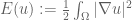
Let us now discuss parabolic PDE in more detail. We begin with a simple example, namely how the heat equation can be used to solve the Dirichlet problem, of constructing a harmonic function 


There are many other settings in geometric topology in which one wants to locate a geometrically structured object (e.g. a harmonic map, a constant-curvature manifold, a minimal surface, etc.) within a certain class (e.g. a homotopy class) by minimising an energy-like functional. In some cases one can achieve this by brute force, creating a minimising sequence and then extracting a limiting object by some sort of compactness argument (as is for instance done in the Sacks-Uhlenbeck theory of minimal 2-spheres), but then one often has little control over the resulting structured object that one obtains in this manner. By using a parabolic flow (as for instance done in the work of Eells-Sampson to obtain harmonic maps in a given homotopy class via harmonic map heat flow) one can often obtain much better estimates and other control on the limit object, especially if certain curvatures in the underlying geometry have a favourable sign.
The most famous recent example of the use of parabolic flows to establish geometric structure from topological objects is, of course, Perelman’s use of the Ricci flow applied to compact 3-manifolds with arbitrary Riemannian metrics, in order to establish the Poincaré conjecture (for the special case of simply connected manifolds) and more generally the geometrisation conjecture (for arbitrary manifolds). [As I understand it, there are some minor but non-trivial technical issues left to clear up with the latter argument, but it seems that these will be resolved soon. The former argument, however, has been checked rather thoroughly.] Perelman’s work showed that Ricci flow, when applied to an arbitrary manifold, will eventually create either extremely geometrically structured, symmetric manifolds (e.g. spheres, hyperbolic spaces, etc.), or singularities which are themselves very geometrically structured (and in particular, their asymptotic behaviour is extremely rigid and can be classified completely). By removing all of the geometric structures that are generated by the flow (via surgery, if necessary) and continuing the flow indefinitely, one can eventually remove all the “pseudorandom” elements of the initial geometry and describe the original manifold in terms of a short list of very special geometric manifolds, precisely as predicted by the geometrisation conjecture. It should be noted that Richard Hamilton had earlier carried out exactly this program assuming some additional curvature hypotheses on the initial geometry; also, when Ricci flow is instead applied to two-dimensional manifolds (surfaces) rather than three, he observed that Ricci flow extracts a constant-curvature metric as its structured component of the original metric, giving an independent proof of the uniformisation theorem (see this recent paper for full details).
Let us now leave parabolic PDE and geometric topology and now discuss Hamiltonian PDE, specifically those of Schrödinger type. (Other classes of Hamiltonian PDE, such as wave or Airy type equations, also exhibit similar features, but we will restrict attention to Schrödinger for sake of concreteness.) These equations formally resemble Hamiltonian ODE, which can be viewed as finite-dimensional measure-preserving dynamical systems with a continuous time parameter 
To illustrate these rather vague assertions, let us first begin with the free linear Schrödinger equation 


which can be interpreted physically as the law of conservation of probability. By using the fundamental solution for this equation, one can also obtain the pointwise decay estimate


and in a similar spirit, we have the local decay estimate


The two properties (*) and (**) may appear contradictory at first, but what they imply is that the solution is dispersing or radiating its (fixed amount of) 

[There is also a very useful and interesting quantitative version of this analysis, known as profile decomposition, in which a solution (or sequence of solutions) to the free linear Schrödinger equation can be split into a small number of “structured” components which are localised in spacetime and in frequency, plus a “pseudorandom” term which is dispersed in spacetime, and is small in various useful norms. These decompositions have recently begun to play a major role in this subject, but it would be too much of a digression to discuss them here. See however my CDM lecture notes for more discussion.]
To summarise so far, for the free linear Schrödinger equation all solutions are radiative or “pseudorandom”. Now let us generalise a little bit by throwing in a (time-independent) potential function 


The famous RAGE theorem of Ruelle, Amrein-Georgescu, and Enss asserts, roughly speaking, that there are no further types of states, and that every state decomposes uniquely into a bound state and a radiating state. For instance, if a solution fails to obey the weak dispersion property (***), then it must necessarily have a non-zero correlation (inner product) with a bound state. (If instead it fails to obey the strong dispersion property (**), the situation is trickier, as there is unfortunately a third type of state, a “singular continuous spectrum” state, which one might correlate with.) More generally, an arbitrary solution will decompose uniquely into the sum of a radiating state obeying (***), and a unconditionally convergent linear combination of bound states. The proof of these facts largely rests on the spectral theorem for the underlying Hamiltonian 
Let us now turn to nonlinear Schrödinger equations. There are a large number of such equations one could study, but let us restrict attention to a particularly intensively studied case, the cubic nonlinear Schrödinger equation (NLS)

where 
- (Global existence) Under what conditions do smooth solutions u to NLS exist globally in time?
- (Asymptotic behaviour, global existence case) If there is global existence, what is the limiting behaviour of u(t) in the limit as t goes to infinity?
- (Asymptotic behaviour, blowup case) If global existence fails, what is the limiting behaviour of u(t) in the limit as t approaches the maximal time of existence?
For reasons of time and space I will focus only on Questions 1 and 2, although question 3 is very interesting (and very difficult). The answer to these questions is rather complicated (and still unsolved in several cases), depending on the sign
- If n = 1, then one has global smooth solutions for arbitrarily large data and any choice of sign.
- For n=2,3,4, one has global smooth solutions for arbitrarily large data in the defocusing case (this is particularly tricky in the energy-critical case n=4), and for small data in the focusing case. For large data in the focusing case, finite time blowup is possible.
- For
, one has global smooth solutions for small data with either sign. For large data in the focusing case, finite time blowup is possible. For large data in the defocusing case, the existence of global smooth solutions are unknown even for spherically symmetric data, indeed this problem, being supercritical, is of comparable difficulty to the Navier-Stokes global regularity problem.
Incidentally, the relevance of the sign

In the defocusing case the Hamiltonian is positive definite and thus coercive; in the focusing case it is indefinite, though in low dimensions and in conjunction with the
Let us now assume henceforth that the solution exists globally (and, to make a technical assumption, also assume that the solution stays bounded in the energy space 
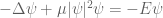
The opposite scenario is that of a nonlinear bound state 


The soliton resolution conjecture asserts that for “generic” choices of (arbitrarily large) initial data to an NLS with a global solution, the long-time behaviour of the solution should eventually resolve into a finite number of receding solitons (i.e. a multisoliton solution), plus a radiation component which decays in senses such as of (**) or (***). (For short times, all kinds of things could happen, such as soliton collisons, solitons fragmenting into radiation or into smaller solitons, etc., and indeed this sort of thing is observed numerically.) This conjecture (which is for instance discussed in the 2006 ICM proceedings article by Soffer, or in some of my own papers) is still far out of reach of current technology, except in the special one-dimensional case n=1 when the equation miraculously becomes completely integrable, and the solutions can be computed rather explicitly via inverse scattering methods, as was for instance carried out by Novoksenov. In that case the soliton resolution conjecture was indeed verified for generic data (in which the associated Lax operator had no repeated eigenvalues or resonances), however for exceptional data one could have a number of exotic solutions, such as a pair of solitons receding at a logarithmic rate from each other, or of periodic or quasiperiodic “breather solutions” which are not of soliton form.
Based on this one-dimensional model case, we expect the soliton resolution conjecture to hold in higher dimensions also, assuming sufficient uniform bounds on the global solution to prevent blowup or “weak turbulence” from causing difficulties. However, the fact that a good resolution into solitons is only expected for “generic” data rather than all data makes the conjecture extremely problematic, as almost all of our tools are based on a worst-case analysis and thus cannot obtain results that are only supposed to be true generically. (This is also a difficulty which seems to obstruct the global solvability of Navier-Stokes, as discussed in an earlier post.) Even in the spherically symmetric case, which should be much simpler (in particular, the solitons must now be stationary and centred at the origin), the problem is wide open.
Nevertheless, there is some recent work which gives a small amount of progress towards the soliton resolution conjecture. For spherically symmetric energy-bounded global solutions (of arbitrary size) to the focusing cubic NLS in three dimensions, it is a result of myself that the solution ultimately decouples into a radiating term obeying (**), plus a “weakly bound state” which is asymptotically orthogonal to all radiating states, is uniformly smooth, and exhibits a weak decay at spatial infinity. If one is willing to move to five and higher dimensions and to weaken the strength of the nonlinearity (e.g. to consider quadratic NLS in five dimensions) then a stronger result is available under similar hypotheses, namely that the weakly bound state is now almost periodic, ranging inside of a fixed compact subset of energy space, thus providing a “dispersive compact attractor” for this equation. In principle, this brings us back to the realm of dynamical systems, but we have almost no control on what this attractor is (though it contains all the soliton states and respects the symmetries of the equation), and so it is unclear what the next step should be. (There is a similar result in the non-radial case which is more complicated to state: see my paper for more details.)

10 comments
Comments feed for this article
10 April, 2007 at 10:24 am
Not Even Wrong » Blog Archive » Math and Physics Roundup
[…] For some more mathematics blogging of the highest possible quality, see Terry Tao’s postings on his Simons lectures at MIT, here, here and here. […]
13 April, 2007 at 10:57 am
stevenm
For parabolic PDE like the heat equation, can one construct entropies to describe these dispersions or flows? In your example, you define the ‘Dirichlet energy’ but is there an entropy that can be constructed and associated with the removal of the random components from the structured components that you described? I think in one of Perelman’s papers he discusses an entropy in connection with the Ricci flow, which seems analogous to heat flow. (Although the details of his papers are beyond my understanding.) A good example of an entropy in Lorentzian (spacetime) geometry would be that associated with black holes and black hole mechanics (leading to Hawking radiation etc.) where an entropy is naturally associated with the area of the horizon, which is a purely geometrical entity.
The algebraic similarity of the heat/diffusion and Schrodinger equation is also quite interesting I think. On a historical note, Schrodinger in 1931 originally considered diffusion processes or Brownian motions, described by the parabolic diffusion/heat equation, as a basis for quantum mechanics. He attempted to formulate Brownian motions in a symmetric form of time reversal, which (supposedly) helped motivate Kolmogorov to pursue some of his own (now classic) work on stochastic processes. But, as you mention, the diffusion/heat equation is not time symmetric whereas quantum theory is, but Schrodinger still felt that quantum theory must be some kind of diffusion or stochastic theory. Feynman’s path integral or sum over paths does also seem to have a very natural interpretation as a sum over mathematical Brownian motions if you make a Wick rotation. I don’t know what the status of this stochastic interpretation and connection with quantum mechanics is these days though.
14 April, 2007 at 6:23 pm
Terence Tao
Dear stevenm,
That is a good question, and I do not know the answer, though given that entropy and the heat equation both show up in thermodynamics, one would expect there to be some sort of connection; presumably it should be known to experts in probability. Certainly the heat flow has many interesting monotonicity properties, especially for non-negative solutions (which are the ones which have a physical Brownian motion interpretation), and I would not be surprised that an entropy-like expression has some nice monotonicity formulae. Perhaps one has to somehow lift the problem to very high dimension (e.g. taking repeated tensor products of the heat flow solution with itself) to see the connection more clearly, as entropy tends to be associated with various asymptotic statistics in the infinite-dimensional limit.
Perelman did introduce an entropy to study Ricci flow (indeed he interpreted Ricci flow as a gradient flow for this entropy), and Hamilton had earlier introduced another entropy-like quantity which also enjoyed a monotonicity property under certain conditions.
It does seem helpful to think of quantum mechanics as a kind of complexified (i.e. Wick rotated) version of classical Brownian motion, in which paths which increase the Hamiltonian are phase rotated rather than damped. There are also some formal similarities between manipulations of bras and kets, and the laws of conditional probability. But as I said before, these analogies seem well suited for understanding the algebraic structure of quantum mechanics, but not its analytic structure.
14 April, 2007 at 7:04 pm
Terence Tao
Actually, now that I think about it, I do know one explicit link between entropy and heat flow: one can interpret the Fisher information of a random variable as the rate of change of the Shannon entropy via heat flow (or more precisely, the Ornstein-Uhlenbeck process, which is basically heat flow renormalised by scaling). I believe this is a useful fact in probability theory, particularly in showing that gaussians are extremisers of various probabilistic quantities, but it is sort of outside my area of expertise.
17 April, 2007 at 4:07 pm
As coisinhas interessantes de hoje… at It’s Equal but It’s Different
[…] Simons Lecture III: Structure and randomness in PDE; […]
13 May, 2008 at 11:04 am
A global compact attractor for high-dimensional defocusing non-linear Schrödinger equations with potential « What’s new
[…] nonlinear Schrödinger equations (NLS). This conjecture (which I also discussed in my third Simons lecture) asserts, roughly speaking, that any reasonable (e.g. bounded energy) solution to such equations […]
7 May, 2009 at 1:13 am
Student
On “the cubic nonlinear Schrödinger equation (NLS)
i u_t + \Delta u = \mu |u|^2 u
where \mu is either equal to +1 (the defocusing case) or -1 (the focusing case).”
I am a novice in Physics. What is the physics reason behind the term focusing and defocusing depending on these signs?
I am also curious to know what you mean by
“weak turbulence.”
Thank you.
7 May, 2009 at 3:58 am
Terence Tao
Dear Student,
One can rewrite the NLS as , where V is the time-dependent potential
  , thus the non-linearity can be viewed as a potential energy component of the Schrodinger operator. A negative value of
  corresponds to a negative
  , i.e. a potential well, which in the linear theory of the Schrodinger equation is known to have an attractive effect. Since V is concentrated where the solution is large, this attractive effect should act to focus the solution. Conversely, a positive value of
  leads to a repulsive potential concentrated at where the solution is large, leading to a defocusing effect.
Weak turbulence is not a term with a commonly agreed upon rigorous definition, but for me it refers to the tendency of solutions of certain evolution equations to shift their energy from low frequencies to high frequencies over extended periods of time, which in particular should cause higher Sobolev norms (e.g. the norm) to grow polynomially in time. In contrast, the turbulent behaviour of equations such as Navier-Stokes results in a more rapid movement of energy from low frequencies to high frequencies, occurring in a bounded amount of time rather than an asymptotic amount, although after that period of turbulence, the dissipative effects tend to kick in and then remove the high-frequency energy from the system. (Establishing this latter fact rigorously is, of course, the $1 million dollar question.)
6 August, 2009 at 8:54 am
Moser’s entropy compression argument « What’s new
[…] in PDE, does have the same algorithm-terminating flavour as the combinatorial arguments; see this earlier blog post for more […]
19 May, 2010 at 8:57 pm
Steffen
This was too much of a coincidence for me not to comment:
It’s interesting that both the heat equation and the Poincaré conjecture made it into the news in the same week that I happened to be browsing this lecture!
http://www.sciencedaily.com/releases/2010/05/100513162755.htm
http://www.claymath.org/poincare/
Keep up the good work! I really enjoy reading your posts!