The crossing number inequality

Today I’d like to discuss a beautiful inequality in graph theory, namely the crossing number inequality. This inequality gives a useful bound on how far a given graph is from being planar, and has a number of applications, for instance to sum-product estimates. Its proof is also an excellent example of the amplification trick in action; here the main source of amplification is the freedom to pass to subobjects, which is a freedom which I didn’t touch upon in the previous post on amplification. The crossing number inequality (and its proof) is well known among graph theorists but perhaps not among the wider mathematical community, so I thought I would publicise it here.

In this post, when I talk about a graph, I mean an abstract collection of vertices V, together with some abstract edges E joining pairs of vertices together. We will assume that the graph is undirected (the edges do not have a preferred orientation), loop-free (an edge cannot begin and start at the same vertex), and multiplicity-free (any pair of vertices is joined by at most one edge). More formally, we can model all this by viewing E as a subset of 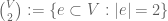, the set of 2-element subsets of V, and we view the graph G as an ordered pair G = (V,E). (The notation is set up so that .)

Now one of the great features of graphs, as opposed to some other abstract maths concepts, is that they are easy to draw: the abstract vertices become dots on a plane, while the edges become line segments or curves connecting these dots. [To avoid some technicalities we do not allow these curves to pass through the dots, except if the curve is terminating at that dot.] Let us informally refer to such a concrete representation D of a graph G as a drawing of that graph. Clearly, any non-trivial graph is going to have an infinite number of possible drawings. In some of these drawings, a pair of edges might cross each other; in other drawings, all edges might be disjoint (except of course at the vertices, where edges with a common endpoint are obliged to meet). If G has a drawing D of the latter type, we say that the graph G is planar.

Given an abstract graph G, or a drawing thereof, it is not always obvious as to whether that graph is planar; just because the drawing that you currently possess of G contains crossings, does not necessarily mean that all drawings of G do. The wonderful little web game “Planarity” illustrates this point excellently. Nevertheless, there are definitely graphs which are not planar; in particular the complete graph on five vertices, and the complete bipartite graph on two sets of three vertices, are non-planar.

There is in fact a famous theorem of Kuratowski that says that these two graphs are the only “source” of non-planarity, in the sense that any non-planar graph contains (a subdivision of) one of these graphs as a subgraph. (There is of course the even more famous four-colour theorem that asserts that every planar graphs is four-colourable, but this is not the topic of my post today.)

Intuitively, if we fix the number of vertices |V|, and increase the number of edges |E|, then the graph should become “increasingly non-planar”; conversely, if we keep the same number of edges |E| but spread them amongst a greater number of vertices |V|, then the graph should become “increasingly planar”. Is there a quantitative way to measure the “non-planarity” of a graph, and to formalise the above intuition as some sort of inequality?

It turns out that there is an elegant inequality that does precisely this, known as the crossing number inequality. It was first discovered by Ajtai-Chvátal-Newborn-Szemerédi and by Leighton (the latter being motivated by optimising VLSI designs). Nowadays it can be proven by two elegant amplifications of Euler’s formula, as we shall see.

If D is a drawing of a graph G, we define cr(D) to be the total number of crossings – where pairs of edges intersect at a point, for a reason other than sharing a common vertex. (If multiple edges intersect at the same point, each pair of edges counts once.) We then define the crossing number cr(G) of G to be the minimal value of cr(D) as D ranges over the drawings of G. Thus for instance cr(G)=0 if and only if G is planar. One can also verify that the two graphs and have a crossing number of 1. This quantity cr(G) will be the measure of how non-planar our graph G is. The problem is to relate this quantity in terms of the number of vertices |V| and the number of edges |E|. We of course do not expect an exact identity relating these three quantities (two graphs with the same number of vertices and edges may have a different number of crossing numbers), so will settle for good upper and lower bounds on cr(G) in terms of |V| and |E|.

How big can the crossing number of a graph G = (V,E) be? A trivial upper bound is cr(G) = O( |E|^2 ), because if we place the vertices in general position (or on a circle) and draw the edges as line segments, then every pair of edges crosses at most once. But this bound does not seem very tight; we expect to be able to find drawings in which most pairs of edges in fact do not intersect.

Let’s turn our attention instead to lower bounds. We of course have the trivial lower bound ; can we do better? Let’s first be extremely unambitious and see when one can get the minimal possible improvement on this bound, namely . In other words, we want to find some conditions on |V| and |E| which will force G to be non-planar. We can turn this around by taking contrapositives: if G is planar, what does this tell us about |V| and |E|?

Here, the natural tool is Euler’s formula |V|-|E|+|F|=2, valid for any planar drawing, where |F| is the number of faces (including the unbounded face). [This is the one place where we shall really use the topological structure of the plane; the rest of the argument is combinatorial.  There are some minor issues if the graph is disconnected, or if there are vertices of degree one or zero, but these are easily dealt with.] What do we know about |F|? Well, every face is adjacent to at least three edges, whereas every edge is adjacent to exactly two faces. By double counting the edge-face incidences, we conclude that . Eliminating |F|, we conclude that for all connected planar graphs with at least one cycle (and this bound is tight when the graph is triangular), which then implies in general. Taking contrapositives, we conclude

whenever . (*)

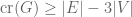
Now, let us amplify this inequality by exploiting the freedom to delete edges. Indeed, observe that if a graph G can be drawn with only cr(G) crossings, then we can delete one of the crossings by removing an edge associated to that crossing, and so we can remove all the crossings by deleting at most cr(G) edges, leaving at least |E|-cr(G) edges (and |V| vertices). Combining this with (*) we see that regardless of the number of crossings, we have

leading to the following amplification of (*):

. (**)

This is not the best bound, though, as one can already suspect by comparing (**) with the crude upper bound 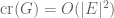. We can amplify (**) further by exploiting a second freedom, namely the ability to delete vertices. One could try the same sort of trick as before, deleting vertices which are associated to a crossing, but this turns out to be very inefficient (because deleting vertices also deletes an unknown number of edges, many of which had nothing to do with the crossing). Indeed, it would seem that one would have to be fiendishly clever to find an efficient way to delete a lot of crossings by deleting only very few vertices.

However, there is an amazing (and unintuitive) principle in combinatorics which states that when there is no obvious “best” choice for some combinatorial object (such as a set of vertices to delete), then often trying a random choice will give a reasonable answer, if the notion of “random” is chosen carefully. (See this paper of Gowers for some further discussion of this principle.) The application of this principle is known as the probabilistic method, first introduced by Erdős.

Here is how it works in this current setting. Let be a parameter to be chosen later. We will randomly delete all but a fraction p of the vertices, by letting each vertex be deleted with an independent probability of 1-p (and thus surviving with a probability of p). Let V’ be the set of vertices that remain. Once one deletes vertices, one also has to delete the edges attached to these vertices; let E’ denote the surviving edges (i.e. the edges connected to vertices in V’). Let G’=(V’,E’) be the surviving graph (known as the subgraph of G induced by V’). Then from (**) we have

.

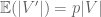
Now, how do we get from this back to the original graph G = (V,E)? The quantities |V’|, |E’|, and cr(G’) all fluctuate randomly, and are difficult to compute. However, their expectations are much easier to compute. Accordingly, we take expectations of both sides (this is an example of the first moment method). Using linearity of expectation, we have

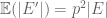
These quantities are all relatively easy to compute. The easiest is . Each vertex in V has a probability p of ending up in V’, and thus contributing 1 to |V’|. Summing up (using linearity of expectation again), we obtain .

The quantity is almost as easy to compute. Each edge e in E will have a probability of ending up in E’, since both vertices have an independent probability of p of surviving. Summing up, we obtain . (The events that each edge ends up in E’ are not quite independent, but the great thing about linearity of expectation is that it works even without assuming any independence.)

Finally, we turn to . Let us draw G in the optimal way, with exactly cr(G) crossings. Observe that each crossing involves two edges and four vertices. (If the two edges involved in a crossing share a common vertex as well, thus forming an shape, one can reduce the number of crossings by 1 by swapping the two halves of the loop in the shape. So with the optimal drawing, the edges in a crossing do not share any vertices in common.) Passing to G’, we see that the probability that the crossing survives in this drawing is only . By one last application of linearity of expectation, the expected number of crossings of this diagram that survive for G’ is . This particular diagram may not be the optimal one for G’, so we end up with an inequality . Fortunately for us, this inequality goes in the right direction, and we get a useful inequality:

.

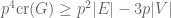
In terms of cr(G), we have

.

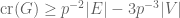
To finish the amplification, we need to optimise in p, subject of course to the restriction , since p is a probability. One can solve the optimisation problem exactly, but we will perform a cheaper computation by settling for a bound which is close to the optimal bound rather than exactly equal to it. A general principle is that optima are often obtained when two of the terms are roughly in balance. A bit of thought reveals that it might be particularly good to have just barely smaller than . (If it is a lot smaller, then p will be large, and we don’t get a good bound on the right. If instead is a lot bigger, then we are likely to have a negative right-hand side.) For instance, we could choose p so that ; this is legal as long as . Substituting this we obtain the crossing number inequality

whenever . (***)

This is quite a strong amplification of (*) or (**) (except in the transition region in which |E| is comparable to |V|).

Is it sharp? We can compare it against the trivial bound , and we observe that the two bounds match up to constants when |E| is comparable to . (Clearly, |E| cannot be larger than .) So the crossing number inequality is sharp (up to constants) for dense graphs, such as the complete graph on n vertices.

Are there any other cases where it is sharp? We can answer this by appealing to the symmetries of (***). By the nature of its proof, the inequality is basically symmetric under passage to random induced subgraphs, but this symmetry does not give any further examples, because random induced subgraphs of dense graphs again tend to be dense graphs (cf. the computation of and above). But there is a second symmetry of (***) available, namely that of replication. If one takes k disjoint copies of a graph G = (V,E), one gets a new graph with k|V| vertices and k|E| edges, and a moment’s thought will reveal that the new graph has a crossing number of k cr(G). Thus replication is a symmetry of (***). Thus, (***) is also sharp up to constants for replicated dense graphs. It is not hard to see that these examples basically cover all possibilities of |V| and |E| for which . Thus the crossing number inequality cannot be improved except for the constants. (The best constants known currently can be found in a recent paper of Pach, Radoicic, Tardos, and Tóth.)

[A general principle, by the way, is that one can roughly gauge the “strength” of an inequality by the number of independent symmetries (or approximate symmetries) it has. If for instance there is a three-parameter family of symmetries, then any example that demonstrates that sharpness of that inequality is immediately amplified to a three-parameter family of such examples (unless of course the example is fixed by a significant portion of these symmetries). The more examples that show an inequality is sharp, the more efficient it is – and the harder it is to prove, since one cannot afford to lose anything (other than perhaps some constants) in every one of the sharp example cases. This principle is of course consistent with my previous post on arbitraging a weak asymmetric inequality into a strong symmetric one.]

— Application: the Szemerédi-Trotter theorem —

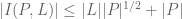
It was noticed by Székely that the crossing number is powerful enough to give easy proofs of several difficult inequalities in combinatorial incidence geometry. For instance, the Szemerédi-Trotter theorem concerns the number of incidences between a finite collection of points P and lines L in the plane. For instance, the three lines and three points of a triangle form six incidences; the five lines and ten points of a pentagram form 20 incidences; and so forth.

One can ask the question: given |P| points and |L| lines, what is the maximum number of incidences I(P,L) one can form between these points and lines? (The minimum number is obviously 0, which is a boring answer.) The trivial bound is , but one can do better than this, because it is not possible for every point to lie on every line. Indeed, if we use nothing more than the axiom that every two points determine at most one line, combined with the Cauchy-Schwarz inequality, it is not hard to show (by double-counting the space of triples such that ) that

. (****)

Dually, using the axiom that two lines intersect in at most one point, we obtain

.

(One can also deduce one inequality from the other by projective duality.)

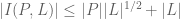
Can one do better? The answer is yes, if we observe that a configuration of points and lines naturally determines a drawing of a graph, to which the crossing number can be applied. To see this, assume temporarily that every line in L is incident to at least two points in P. A line l in L which is incident to k points in P will thus contain k-1 line segments in P; k-1 is comparable to k. Since the sum of all the k is I(P,L) by definition, we see that there are roughly I(P,L) line segments of L connecting adjacent points in P; this is a diagram with |P| vertices and roughly |I(P,L)| edges. On the other hand, a crossing in this diagram can only occur when two lines in L intersect. Since two lines intersect in at most one point, the total number of crossings is O(|L|^2). Applying the crossing number inequality (***), we obtain

if I(P,L) is much larger than |P|

which leads to

.

We can then remove our temporary assumption that lines in L are incident to at least two points, by observing that lines that are incident to at most one point will only contribute O(|L|) incidences, leading to the Szemerédi-Trotter theorem

.

This bound is somewhat stronger than the previous bounds, and is in fact surprisingly sharp; a typical example that demonstrates this is when P is the lattice and L is the set of lines with slope and intercept ; here and the number of incidences is roughly .

The original proof of this theorem, by the way, proceeded by amplifying (****) using the method of cell decomposition; it is thus somewhat similar in spirit to Szekély’s proof, but was a bit more complicated technically. Wolff conjectured a continuous version of this theorem for fractal sets, sometimes called the Furstenberg set conjecture, and related to the Kakeya conjecture; a small amount of progress beyond the analogue of (****) is known, thanks to work of Katz and myself and of Bourgain, but we are still far from the best possible result here.

— Application: sum-product estimates —

One striking application of the Szemerédi-Trotter theorem (and by extension, the crossing number inequality) is to the arena of sum-product estimates in additive combinatorics, which is currently a very active area of research, especially in finite fields, due to its connections with some long-standing problems in analytic number theory, as well as to some computer science problems concerning randomness extraction and expander graphs. However, our focus here will be on the more classical setting of sum-product estimates in the real line .

Let A be a finite non-empty set of non-zero real numbers. We can form the sum set

and the product set

.

If A is in “general position”, it is not hard to see that and both have cardinality comparable to . However, in certain cases one can make one or the other sets significantly smaller. For instance, if A is an arithmetic progression , then the sum set has cardinality comparable to just |A|. Similarly, if A is a geometric progression , then the product set has cardinality comparable to |A|. But clearly A cannot be an arithmetic progression and a geometric progression at the same time (unless it is very short). So one might conjecture that at least one of the sum set and product set should be significantly larger than A. Informally, this is saying that no finite set of reals can behave much like a subring of .

This intuition was made precise by Erdős and Szemerédi, who established the lower bound

for some small which they did not make explicit. They then conjectured that in fact c should be made arbitrary close to the optimal value of 1, and more precisely that

for large |A| and some absolute constant .

The Erdős-Szemerédi conjecture remains open, however the value of c has been improved; currently, the best bound is due to Solymosi, who showed that c can be arbitrarily close to 3/11. Solymosi’s argument is based on an earlier argument of Elekes, who obtained c=1/4 by a short and elegant argument based on the Szemerédi-Trotter theorem which we will now present. The basic connection between the two problems stems from the familiar formula y=mx+b for a line, which clearly encodes a multiplicative and additive structure. We already used this connection implicitly in the example that demonstrated that the Szemerédi-Trotter theorem was sharp. For Elekes’ argument, the challenge is to show that if and are both small, then a suitable family of lines associated to A will have a high number of incidences with some set of points associated to A, so that the Szemerédi-Trotter may then be profitably applied. It is not immediately obvious exactly how to do this, but Elekes settled upon the choice of letting , and letting L be the space of lines y=mx+b with slope in and intercept in A, thus and . One observes that each line in L is incident to |A| points in P, leading to incidences. Applying the Szemerédi-Trotter theorem and doing the algebra one eventually concludes that . (A more elementary proof of this inequality, not relying on the Szemerédi-Trotter theorem or crossing number bounds, and thus having the advantage on working on other archimedean fields such as , was subsequently found by Solymosi, but the best bounds on the sum-product problem in still rely very much on the Szemerédi-Trotter inequality.)