Given a positive integer  , let
, let  denote the number of divisors of n (including 1 and n), thus for instance d(6)=4, and more generally, if n has a prime factorisation
 (1)
(1)
then (by the fundamental theorem of arithmetic)
 . (2)
. (2)
Clearly,  . The divisor bound asserts that, as gets large, one can improve this trivial bound to
 (3)
(3)
for any  , where
  depends only on
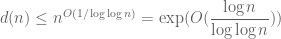
  ; equivalently, in asymptotic notation one has
  . In fact one has a more precise bound
 . (4)
. (4)
The divisor bound is useful in many applications in number theory, harmonic analysis, and even PDE (on periodic domains); it asserts that for any large number n, only a “logarithmically small” set of numbers less than n will actually divide n exactly, even in the worst-case scenario when n is smooth. (The average value of d(n) is much smaller, being about  on the average, as can be seen easily from the double counting identity
 ,
,
or from the heuristic that a randomly chosen number m less than n has a probability about 1/m of dividing n, and  . However, (4) is the correct “worst case” bound, as I discuss below.)
The divisor bound is elementary to prove (and not particularly difficult), and I was asked about it recently, so I thought I would provide the proof here, as it serves as a case study in how to establish worst-case estimates in elementary multiplicative number theory.
[Update, Sep 24: some applications added.]
— Proof of (3) —
Let’s first prove the weak form of the divisor bound (3), which is already good enough for many applications (because a loss of  is often negligible if, say, the final goal is to extract some polynomial factor in n in one’s eventual estimates). By rearranging a bit, our task is to show that for any , the expression
 (5)
(5)
is bounded uniformly in n by some constant depending on . Using (1) and (2), we can express (5) as a product
 (6)
(6)
where each term involves a different prime  , and the
  are at least 1. We have thus “localised” the problem to studying the effect of each individual prime independently. (We are able to do this because d(n) is a multiplicative function.)
Let’s fix a prime and look at a single term  . The numerator is linear in , while the denominator is exponential. Thus, as per Malthus, we expect the denominator to dominate, at least when is large. But, because of the , the numerator might be able to exceed the denominator when is small – but only if is also small.
Following these heuristics, we now divide into cases. Suppose that is large, say  . Then
  (by Taylor expansion), and so the contribution of to the product (6) is at most 1. So all the large primes give a net contribution of at most 1 here.
What about the small primes, in which  ? Well, by Malthus, we know that the sequence
  goes to zero as
  . Since convergent sequences are bounded, we therefore have some bound of the form
  for some
  depending only on and , but not on . So, each small prime gives a bounded contribution to (6) (uniformly in n). But the number of small primes is itself bounded (uniformly in n). Thus the total product in (6) is also bounded uniformly in n, and the claim follows.
— Proof of (4) —
One can refine the above analysis to get a more explicit value of , which will let us get (4), as follows.
Again consider the product (6) for some . As discussed previously, each prime larger than  gives a contribution of at most 1. What about the small primes? Here we can estimate the denominator from below by Taylor expansion:

and hence

(the point here being that our bound is uniform in ). One can of course use undergraduate calculus to try to sharpen the bound here, but it turns out not to improve by too much, basically because the Taylor approximation  is quite accurate when x is small, which is the important case here.
Anyway, inserting this bound into (6), we see that (6) is in fact bounded by

Now let’s be very crude and bound  from below by
  , and bound the number of primes less than by . (One can of course be more efficient about this, but again it turns out not to improve the final bounds too much. A general principle is that when one estimating an expression such as
  , or more generally the product of B terms, each of size about A, then it is far more important to get a good bound for B than to get a good bound for A, except in those cases when A is very close to 1.) We thus conclude that
 ;
;
unwinding what this means for (3), we obtain

for all  and . If we now set
  for a sufficiently large C, then the second term of the RHS dominates the first (as can be seen by taking logarithms), and the claim (4) follows.
The above argument also suggests the counterexample that will demonstrate that (4) is basically sharp. Pick , and let n be the product of all the primes up to . The prime number theorem tells us that  . On the other hand, the prime number theorem also tells us that the number of primes dividing n is
  , so by (2),
  . Using these numbers we see that (4) is tight up to constants. [If one does not care about the constants, then one does not need the full strength of the prime number theorem to show that (4) is sharp; the more elementary bounds of Chebyshev, that say that the number of primes up to N is comparable to
  up to constants, would suffice.]
— Why is the divisor bound useful? —
One principal application of the divisor bound (and some generalisations of that bound) is to control the number of solutions to a Diophantine equation. For instance, (3) immediately implies that for any fixed positive n, the number of solutions to the equation

with x,y integer, is only at most. (For x and y real, the number of solutions is of course infinite.) This can be leveraged to some other Diophantine equations by high-school algebra. For instance, thanks to the identity  , we conclude that the number of integer solutions to

is also at most ; similarly, the identity  implies that the number of integer solutions to

is at most . (Note from Bezout’s theorem (or direct calculation) that  and
and  determine
  up to at most a finite ambiguity.)
Now consider the number of solutions to the equation
 .
.
In this case,  does not split over the rationals
  , and so one cannot directly exploit the divisor bound for the rational integers
  . However, we can factor
  over the Gaussian rationals
 ![{\Bbb Q}[\sqrt{-1}]](https://s0.wp.com/latex.php?latex=%7B%5CBbb+Q%7D%5B%5Csqrt%7B-1%7D%5D&bg=ffffff&fg=545454&s=0&c=20201002) . Happily, the Gaussian integers
. Happily, the Gaussian integers ![{\Bbb Z}[\sqrt{-1}]](https://s0.wp.com/latex.php?latex=%7B%5CBbb+Z%7D%5B%5Csqrt%7B-1%7D%5D&bg=ffffff&fg=545454&s=0&c=20201002) enjoy essentially the same divisor bound as the rational integers ; the Gaussian integers have unique factorisation, but perhaps more importantly they only have a finite number of units (
enjoy essentially the same divisor bound as the rational integers ; the Gaussian integers have unique factorisation, but perhaps more importantly they only have a finite number of units ( to be precise). Because of this, one can easily check that
  also has at most solutions.
One can similarly exploit the divisor bound on other number fields; for instance the divisor bound for ![{\Bbb Z}[\sqrt{-3}]](https://s0.wp.com/latex.php?latex=%7B%5CBbb+Z%7D%5B%5Csqrt%7B-3%7D%5D&bg=ffffff&fg=545454&s=0&c=20201002) lets one count solutions to
lets one count solutions to  or
or  . On the other hand, not all number fields have the divisor bound. For instance,
 ![{\Bbb Z}[\sqrt{2}]](https://s0.wp.com/latex.php?latex=%7B%5CBbb+Z%7D%5B%5Csqrt%7B2%7D%5D&bg=ffffff&fg=545454&s=0&c=20201002) has an infinite number of units, which means that the number of solutions to Pell’s equation
has an infinite number of units, which means that the number of solutions to Pell’s equation

is infinite.
Another application of the divisor bound comes up in sieve theory. Here, one is often dealing with functions of the form  , where the sieve weights
  typically have size
  , and the sum is over all d that divide n. The divisor bound (3) then implies that the sieve function
  also has size . This bound is too crude to deal with the most delicate components of a sieve theory estimate, but is often very useful for dealing with error terms (especially those which have gained a factor of
  relative to the main terms for some
  ).
).


46 comments
Comments feed for this article
23 September, 2008 at 3:37 pm
Anonymous Rex
Is the constant known in (4) as it is in the prime number theorem?
23 September, 2008 at 6:39 pm
bengreen
Terry,
The divisor bound is indeed surprisingly powerful, and is a good way of importing the information contained in the unique factorization theorem for the integers into analytic number theory (and other subjects, as you remark). It is always nice when some algebraic theory gives a highly portable tool that us analysts can use; another example would be the Weil bound for Kloosterman sums.
A good example in analytic number theory where the use of the divisor bound is critical is Hua’s result placing a good upper bound on the number of solutions to with
with  , provided that
  . One may read about this in Vaughan’s book on the Hardy-Littlewood method.
I only recently came to realise how subtle the bound is, when I found myself wishing for a similar-looking estimate. Let be some fixed number (say
  ). We say that
  is a generalised divisor of
  if there is some
  such that
  . So one is trying to do a kind of generalised arithmetic, in which the integers have been shifted by
  . Can you show that
  has
has  generalised divisors, perhaps even uniformly in the choice of
  ?
?
I pretty soon realised that there is no sensible theory of factorisation for these generalised integers, and then I found another way to tackle the problem I was actually interested in. Still, I would be interested to see a solution to this question!
I asked Roger Heath-Brown about the divisor function estimate, and he said that the best bounds known by “robust” methods are something like . He mentioned something about a paper of Bombieri and Pila but I forget the details.
One more thing – it is perhaps worth remarking (not to you in particular, as we have used this in a couple of our papers :-) ) that if one only wants an bound then it is possible to do better. Namely,
where I think one can take
Enjoy the rest of your two-week hiatus
Ben
23 September, 2008 at 9:06 pm
Emmanuel Kowalski
Indeed, the higher moments are given by
for any fixed integer (and it does work also with arbitrary complex values of
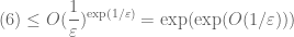
  , or at least with positive real part — one has to look at the Selberg-Delange method to see if all complex
  are possible). The exponential growth of the exponent
  is another indication that large values of the divisor function are not so infrequent.
I think it was Ramanujan who first gave an elementary proof of these estimates, but nowadays it’s probably simpler to see it as a special case of general results on sums of multiplicative functions. The exponent is because
  (the
(the  comes from summing
  instead of
  ).
).
11 February, 2018 at 9:33 am
John Espino
Would you be able to provide more information on where I can find this relation?
23 September, 2008 at 9:51 pm
Marius Overholt
The constant in (4) is . This is due to the Swedish mathematician Severin Wigert around 1908. There is a multiplicative constant
  in Ramanujan’s asymptotic relation for the summatory function of
  , for example
23 September, 2008 at 10:00 pm
Harald Hanche-Olsen
On a (much) lighter note, I enjoyed (and was startled by) the reference to Malthus that you casually threw in there. As I teach elementary calculus this year, I have an opportunity to steal this idea in order to enliven the subject a bit.
23 September, 2008 at 11:19 pm
Emmanuel Kowalski
Yes, I had indeed forgotten the leading constant in the asymptotic formula of Ramanujan…
I just checked in Tenenbaum’s book that, as suspected, there is an asymptotic formula (with suitable leading constant again) for all complex powers of .
.
24 September, 2008 at 2:07 am
The Anonymous
Not that much related – but enjoyable. Given a positive integer , construct recursively a sequence with the first term
  and
and What is the set of those
 such that this sequence does not contain a square?
each subsequent term equal to the number of divisors of the previous
term:
22 March, 2017 at 1:39 pm
Anonymous
Null set ! it will eventually end with a 2 , and if the term before is an odd prime ,it has definitely from a perfect square …
24 September, 2008 at 6:41 pm
PDE
Prof. Tao:
Could you give a more specific application of the divisor bound in PDEs?
Many thanks.
25 September, 2008 at 7:16 am
Giovanni
Dear Prof. Tao
What do you think about a relation with p-adic analysis ?
Best regards
25 September, 2008 at 4:44 pm
Jaime Montuerto
Jaime Montuerto
Prime Number Distributions
26 Sept 2008
Dear Terry and Ben,
I have a hypothesis that might interest you both and related to this area. I have been interested in factoring algorithms and
related areas in number theory, although I’m not sure how elementary or obvious it might seem because there are so many
references about this. I do not know how to write this in the formalized way that you all are familiar with so please bear with me
about this. So I will call it a hypothesis.
The hypothesis is that every Mersenne number has at least one prime number in a one-to-one mapping with it and that the caliper signature (my term, explained below) of that prime number is the order of the Mersenne. Putting it differently, every prime number divides a unique smallest mersenne and the definition of caliper signature is the order of that mersenne.
A prime Mersenne number is the actual prime itself. A composite Mersenne would have at least two factors or more. The special prime number in question has a unique property compared to the rest of the prime factors.
This caliper signature is a function very much related to Euler totient functions and Carmichael functions with a subtle but very important difference. The analysis is done in binary numbers or multiple of 2’s. This is where this function makes sense and also applies only to odd numbers. To handle even numbers, you just factor out the 2^k factor and consider the odd factor for analysis.
Here are some of the related properties of the Caliper Signature (J): (Note: the equal sign is actually a congruence relation)
a^(p-1) = 1 (mod p) By Fermat
a^phi(p) = 1 (mod p) By Euler
a^Y(p) = 1 (mod p) By Carmichael early 20th
2^phi(p) = 1 (mod p) By Boniakovsky 19th
2^J(p) = 1 (mod p) the Caliper Signature Hypothesis.
1) J(p) | phi(p) Then a prime number or pseudoprimes. And an extra test for pseudoprimes and carmichael numbers.
2) J(abc..) = LCM{a,b,c,…} This is similar to Carmichael numbers for the composite numbers.
3) J(a^e1 * b^e2 * c^e3 * …) = LCM{J(a),a^(e1-1),J(b),b^(e2-1),J(c),c^(e3-1),….}
Again this is different from both totient and Carmichael functions.
3) J(Mersenne) = order or width of the Mersenne.
This is where it differs from both totient and carmichael functions, the caliper signature is half of both. This is can be done by algorithmic calculation. There are several algorithms I have been developing.
4) Algorithm for calculating Caliper Signature of an integer, N.
I think this is the simplest and elegant one, and though it’s not the most efficient it’s a beautiful algorithm. The remainders will cycle back to 1.
a) Starting from 1 as first remainder, double it.
b) If the result is more than N, subtract/remove N. This is the mod operation.
c) Double again the resulting remainder.
d) Repeat the process until the remainder 1 is reached. This is the end of the cycle.
e) Count the number of processes or doublings, and that is the Caliper Signature.
e.g. I used the convention of starting at the right side as LSB (least significant bit). Also the number Mersenne 4 (M4) is the order not the actual value. So 7 is M3, where the 3 is the caliper signature or the order of mersenne.
N= 11 J= 10 12->1,6,14->3,18->7,20->9,10,16->5,8,4,2,1
{1,6,3,7,9,10,5,8,4,2,1}
N= 15 J= 4 {1,8,4,2,1}
N= 3 J= 2 {1,2,1}
Both 3 and 5 are factors of M4 = 15 but only 5 has
N= 5 J= 4 {1,4,2,1}
N= 23 J= 11 {1,12,6,3,13,18,9,16,8,4,2,1}
N= 89 J= 11 {1,45,67,78,39,64,32,16,8,4,2,1}
N= 7 J= 3 {1,4,2,1}
N= 17 J= 8 {1,9,13,15,16,8,4,2,1} This is Fermat number.
Fermat numbers have a special quick formulation J(Fermat number,Fn= a^n + 1) = 2*n.
Applications of Caliper Signature:
The caliper signature has deeper connections with number theory. Its binary number operation is important because there is an inherent property that does not appear in other number systems, though this id not saying that other bases or models are not important. First it makes sense only in the binary system, but importantly this system shows, I believe, natural formation and patterns of properties let alone the one-to-one mapping of the binary system to the number system.
Some of the most important properties of this hypothesis are the determination of primes distribution, the calculations of numbers of divisors, primality tests specially on pseudo primes and carmichael numbers test and possibly binary bits compression.
A. PRIME NUMBER DISTRIBUTION:
Mersenne numbers are so vital and central to this hypothesis. Such that every prime number is linked to a specific Mersenne so that, given a mersenne, there is an algorithmic process to find THE prime number and vice versa. This might shed light on the enigma of prime distributions. It’s explicit in the hypothesis that ALL mersennes give off one or more primes, and there is a one-to-one mapping of this relationship. Every prime number is mapped singly to a specific mersenne but not the other way around. Mersenne M11 gives 23 and 89 as prime numbers. So both 23 and 89 have caliper signature of 11 (see above example). Importantly, not all prime factors of composite mersennes have the same caliper signature of the mersenne. The prime factor/s that have caliper signatures of the order of mersenne are the ones of interest in the prime distribution.
Since all primes are linked to a specific mersenne, it follows then that the distribution of prime numbers is directly linked to the distribution of all mersennes in progression. The progression of mersennes is a recurrence relation that is Mnext = 2*Mprevious + 1, 15 = 2*7 + 1. This distribution of mersennes fits neatly to the statistic distribution, prime number theorem and Gauss estimates of logx. Now what’s really interesting is that the ordering of values of primes does not follow the ordering sizes of its corresponding mersennes. Sometimes a bigger mersenne has a much lower prime association than a few order smaller mersennes. This behaviour that made the prime distribution seems paradodixal and chaotic. And this mechanism explains why twin primes and clustering of primes are possible. Again the relationship of neighboring mersennes doubles its neighbor but the primes lag more often to its
mersennes. Some mersennes have several primes and perhaps as the mersenne get bigger, it might have more primes in it, and this affects the density of primes, given a range.
TERRY, when you were here last at SYdney University a few months ago giving your lecture, I was honored to meet and talk to you/ In fact I tried to explain this to you at that time but everyone was wanting to talk to you and there was not time to explain fully. Though I was pleased to be able to canvas what I did at the time. I tried to show the list of first set of mersennes with their corresponding primes.
And here it is – a very small list but.
Mersenne -> the prime number link.
{M1=>1, M2=>3, M3->7, M4->5, M5->31, M6->* (strictly 3), M7->127, M8->17, M9->73, M10->11, M11->23 and 89,
M12->13, M13->8191, M14->43, M15->151, M16->257, M17->131071, M18->19, M19->524287, M20->41, M21->337, M22->683,
M23->47, M24->241, M25->601 and 1801, M26->2731, M27->262657, M28->29 and 113, M29->233, M30->331, ….}
I have been isolated about this for quite a while and it’s good to share this, specially on your blog. Thanks for this and I hope for any comments, corrections, questions and any other verifications that you feel you could make.
Thanks in anticipation
Jaime Montuerto
26 September, 2008 at 7:19 am
Gergely Harcos
The precise bound was first proved by Wigert in 1906 using the prime number theorem, while Ramanujan in 1914 observed its elementary character. In fact we can prove the inequality even without knowing unique factorization! All we need to know is that
  and
and  imply
imply  . This property implies
  as one can inject the set of divisors of
  into the set of pairs formed of a divisor of
  and a divisor of
  : to
: to  assign the pair
  . Once we know
  we can see for any positive integer
  that
that  . It follows that
  , whence also
  . Now the second exponent
  changes by a factor less than 2 whenever
  is increased by 1, so we can certainly find a
  with
with  . This choice furnishes Wigert’s estimate upon observing that
  .
.
26 September, 2008 at 10:38 am
Terence Tao
Dear Ben,
Your question is very close to that of counting lattice points on (or very close to) a generic curve (in this case, a hyperbola). There is an example of Jarnik of a curve in![{}[1,N] \times [1,N]](https://s0.wp.com/latex.php?latex=%7B%7D%5B1%2CN%5D+%5Ctimes+%5B1%2CN%5D&bg=ffffff&fg=545454&s=0&c=20201002) that passes through about
that passes through about  lattice points despite having curvature uniformly bounded from below, so in analogy to this, I would not expect any bounds better than
  for your problem (given that the hyperbola
  spends some time in a square of length about
  ) without using some additional arithmetic structure in the problem (if such exists).
Dear PDE,
The divisor bound is used to establish type bounds for solutions to linear PDE on periodic domains (and hence to certain nonlinear PDE, by standard perturbation theory techniques). This was noticed in particular by Bourgain around 1991. As an example, a periodic solution to the Airy equation
  takes the form
  . Typically, one has
  type control on
  , which by Plancherel’s theorem leads to
  type control on the coefficients
  . If one wished to compute, say, the
  norm of u (say on a bounded time interval), standard Fourier analysis and Cauchy-Schwarz manipulations eventually lead one to controlling the multiplicity of solutions
  to the problem
  ,
,  for various a, b. It turns out that by some high school algebra similar to that at the end of my post, and in particular by using the identity
one can control this multiplicity using the divisor bound.
28 September, 2008 at 12:05 pm
anonymous
Is there a geometric analog of the divisor bound for curves over finite fields? E.g. a way to bound the no. of ideals that contain a given polynomial.
29 September, 2008 at 6:23 am
The divisor bound ( from T.Tao ’s blog ) « Khatuanminh’s Weblog
[…] 23 September, 2008 at 6:39 pm […]
7 February, 2009 at 5:35 am
Dilettante Arithmetician
Prof. Tao,
I am a graduate student and found this article very informative. I am getting a taste of analytic number theory from your and Kowalski’s blogs.
I would be indebted to you if it is possible for you to write up a similar blog post about the Weil bound for Kloosterman sums, in a similar lucid style.
Thanks,
g.
17 August, 2010 at 3:31 am
Raitis
Does anybody know better estimates of than classical S. Wigert’s result obtained in 1906? Thank you!
1 November, 2010 at 11:03 am
Eytan Paldi
Better estimates for d(n) appear in my MSC thesis (from 1984) at the Technion. For example, by the exponent
 is less than
where c=2 is permissible but can’t be reduced to c=1.93
Moreover, by assuming Riemann hypothesis, an asymptotic expansion for the exponent in terms of negative powers of log log n where derived.
Similarly, the constant
where c=3 is permissible but can’t be reduced to c=2.795
Related information may be found in the doctoral thesis (from 1983) of Guy Robin.
3 November, 2010 at 8:52 am
Eytan Paldi
Some corrections to my last comment:
1. should be replaced by
  .
.
2. The asymptotic expansion for the exponent was found by an elementary method (using only the prime number theorem with simple remainder term) in terms of powers of
  – also by an elementary method.
Similar asymptotic expansion was found for
By assuming Riemann hypothesis, only the remainder term can be improved.
3. The first (analytic) proof for asymptotic expansions (with remainder term) for sums of powers of d(n) was apparently given by B. M. Wilson in his paper “Proofs of some formulae enunciated by Ramanujan” Proc. London Math. Soc. (2) 21 (1922), 235-255.
6 November, 2010 at 8:52 am
Raitis Ozols
Thank You!
7 July, 2011 at 10:52 am
On the number of solutions to 4/p = 1/n_1 + 1/n_2 + 1/n_3 « What’s new
[…] familiar with analytic number theory will recognise the right-hand side from the divisor bound, which indeed plays a role in the […]
23 July, 2011 at 7:41 pm
Erdos’ divisor bound « What’s new
[…] of some error terms in the proof of (6). These should be compared with what one can obtain from the divisor bound and the trivial bound , giving the […]
31 July, 2011 at 10:17 pm
Counting the number of solutions to the Erdös-Straus equation on unit fractions « What’s new
[…] torsor of the Cayley surface.) By optimising between these parameterisations and exploiting the divisor bound, we obtain some bounds on the worst-case behaviour of and , […]
16 December, 2011 at 10:15 am
254B, Notes 3: Quasirandom groups, expansion, and Selberg’s 3/16 theorem « What’s new
[…] such , the number of with and is . For each fixed and , the expression is of size ; by the divisor bound, there are thus ways to factor into . Thus, we obtain a final bound […]
16 December, 2011 at 10:53 am
254B, Notes 3: Quasirandom groups, expansion, and Selberg’s 3/16 theorem | t1u
[…] such , the number of with and is . For each fixed and , the expression is of size ; by the divisor bound, there are thus ways to factor into . Thus, we obtain a final bound […]
18 September, 2012 at 2:56 pm
The probabilistic heuristic justification of the ABC conjecture « What’s new
[…] to apply probabilistic heuristics to. For Step 3, we need the following lemma, reminiscent of the classical divisor bound: Lemma 3 Let be a square-free integer. Then there are at most integers less than with radical […]
16 April, 2013 at 11:30 am
Anonymous
What’s known about the estimate on d(n, Q), the number of divisors of n less than Q? Thank you.
10 June, 2013 at 5:33 pm
A combinatorial subset sum problem associated with bounded prime gaps | What's new
[…] (i.e. a Brun-Titchmarsh type inequality for powers of the divisor function); this estimate follows from this paper of Shiu or this paper of Barban-Vehov, and can also be proven using the methods in this previous blog post. (The factor of is needed to account for the possibility that is not primitive, while the term accounts for the possibility that is as large as .) Finally, (16) follows from the standard divisor bound; see this previous post. […]
12 June, 2013 at 1:03 pm
Estimation of the Type I and Type II sums | What's new
[…] and similarly (using the crude divisor bound) […]
22 June, 2013 at 7:38 am
Bounding short exponential sums on smooth moduli via Weyl differencing | What's new
[…] , and said to be bounded if . Another convenient notation: we write for . Thus for instance the divisor bound asserts that if has polynomial size, then the number of divisors of is […]
18 October, 2014 at 4:32 am
A New Provable Factoring Algorithm | Gödel's Lost Letter and P=NP
[…] “” hides sub-linear terms including coming from the divisor bound, logarithmic terms from the overhead in nearly-linear time integer multiplication, and related […]
16 February, 2015 at 11:25 am
hiklicepleh
Dear Terence Tao,

 – number of divisors of
  .
.


Without assuming the Riemann hypothesis, Robin revealed –
for all
Now apply some tricks.
And finally,
16 February, 2015 at 10:37 pm
hiklicepleh
Not sure where the error is. Could you tell?
17 February, 2015 at 7:47 am
Terence Tao
There is an n missing in the last line, but more importantly, the inequalities do not go the right way ( and
and  do not imply
  ).
).
23 April, 2015 at 11:54 am
Quora
What are some tight upper bounds on the number of factors of a number [math]n[/math]?
Yes, we can do much better. Let [math]d(n)=\sum_{d|n}1[/math] be the number of divisors of [math]n[/math]. Then not only is this number less than [math]n^{1/2}[/math] as you suggested, it is in fact less than [math]n^\epsilon[/math] any positive [mat…
4 August, 2015 at 8:47 am
gninrepoli
What about the upper bound for the ?
?
26 August, 2015 at 7:19 pm
Heath-Brown’s theorem on prime twins and Siegel zeroes | What's new
[…] if one replaces with for . For fixed , the number of such pairs is at least , thanks to the divisor bound. Thus it will suffice to establish the fourth moment […]
11 September, 2015 at 6:27 am
The Erdos discrepancy problem via the Elliott conjecture | What's new
[…] or , the inner sum is , which by the divisor bound gives a negligible contribution. Thus we may restrict to . Note that as is already restricted to […]
11 December, 2015 at 4:51 pm
The two-dimensional case of the Bourgain-Demeter-Guth proof of the Vinogradov main conjecture | What's new
[…] when combined with the divisor bound, shows that each is associated to choices of excluding diagonal cases when two of the collide, […]
4 November, 2018 at 12:50 am
Sean Eberhard
What about a bound for the number of divisors of
  of size at most
  ? Given that
  , I would expect to get a nontrivial bound whenever
  is much smaller than
  .
.
2 December, 2019 at 6:07 pm
Anonymous
Dear Prof. Tao,
Here is how I am looking at the argument:
1) The divisors formed from large primes (primes> log n) are at most exp( logn/loglogn) –because there are at most logn/loglogn such prime factors. This corresponds to your truncation $p> exp(1/\epsilon)$
2) And for small primes also you get the same bound. But in your argument, this happens by comparing with n^\epsilon where you start with d(n)/n^\epsilon and show that these quantities are bounded by 1/epsilon logp and using mutliplicativity.
If I want to bound it without the comparison with the n^{\epsilon}, what kind of argument do we need to deal with the small primes?
If I can somehow argue that the worst case is when you have product of all these small primes, –you have logn/loglogn of them and hence the number of divisors is exp(O(logn/loglogn). But in the prime factorization there could be a high multiplicity of say very small primes by sacrificing a slightly large prime, or a high multiplicity for a prime by sacrificing a lot of small primes and these cases might potentially give more divisors.(Not true, but how do we see this?)
How do you think we can see this? Basically I want to “see” the following part of the bound without the comparison with n^{epsilon} and somehow directly argue that divisors from small prime factors are not too many. (I need this for reasons having to deal with “level” lowering trick in a problem involving divisors– I want to know how these n^{\epsilon} is “seeing” the small prime factors of n )
$$\displaystyle \frac{a_j+1}{p_j^{\varepsilon a_j}} \leq \frac{a_j+1}{1+\varepsilon a_j \log p_j} \leq O( \frac{1}{\varepsilon \log p_j} )” title=”\displaystyle \frac{a_j+1}{p_j^{\varepsilon a_j}} \leq \frac{a_j+1}{1+\varepsilon a_j \log p_j} \leq O( \frac{1}{\varepsilon \log p_j} )$$
2 December, 2019 at 6:28 pm
Anonymous
We could just say that we bound (k+1) by loglogn/log p p^{k/loglogn} — and then apply multiplicativity– But what does this bound mean? Why are bounding the divisors from a fixed prime factor in terms of a quantity that again involving the contribution from the prime factor ? 9Yes, the bounds multiply to become n^{1/loglogn}– but still– what is happening here? What kind of argument is it?
26 February, 2020 at 7:17 am
Marcelo Nogueira
Dear Prof. Tao, as discussed above, to get satisfactory bounds ,
,  , is a complicated problem.
(i.e., of the form
It is possible to use some idea by mean of the above?
Decoupling Theorems (Bourgain-Demeter) to obtain satisfactory bounds to the sets
26 February, 2020 at 7:22 am
Anonymous
Remark:
where
23 December, 2022 at 12:39 am
asymptotic form of divisor bound – Mathematics – Forum
[…] $d(n)$ denote the divisor function, the number of divisors of $n$. Following this post of Tao, https://terrytao.wordpress.com/2008/09/23/the-divisor-bound/ I have managed to show that $d(n) leq C_{epsilon}n^{epsilon}$ for any $epsilon > […]