Heath-Brown’s theorem on prime twins and Siegel zeroes

26 August, 2015 in expository, math.NT | Tags: prime numbers, Roger Heath-Brown, Siegel zero, twin primes | by Terence Tao

The twin prime conjecture is one of the oldest unsolved problems in analytic number theory. There are several reasons why this conjecture remains out of reach of current techniques, but the most important obstacle is the parity problem which prevents purely sieve-theoretic methods (or many other popular methods in analytic number theory, such as the circle method) from detecting pairs of prime twins in a way that can distinguish them from other twins of almost primes. The parity problem is discussed in these previous blog posts; this obstruction is ultimately powered by the Möbius pseudorandomness principle that asserts that the Möbius function ${\mu}$ is asymptotically orthogonal to all “structured” functions (and in particular, to the weight functions constructed from sieve theory methods).

However, there is an intriguing “alternate universe” in which the Möbius function is strongly correlated with some structured functions, and specifically with some Dirichlet characters, leading to the existence of the infamous “Siegel zero“. In this scenario, the parity problem obstruction disappears, and it becomes possible, in principle, to attack problems such as the twin prime conjecture. In particular, we have the following result of Heath-Brown:

Theorem 1 At least one of the following two statements are true:

(Twin prime conjecture) There are infinitely many primes ${p}$ such that ${p+2}$ is also prime.
(No Siegel zeroes) There exists a constant ${c>0}$ such that for every real Dirichlet character ${\chi}$ of conductor ${q > 1}$ , the associated Dirichlet ${L}$ -function ${s \mapsto L(s,\chi)}$ has no zeroes in the interval ${[1-\frac{c}{\log q}, 1]}$ .

Informally, this result asserts that if one had an infinite sequence of Siegel zeroes, one could use this to generate infinitely many twin primes. See this survey of Friedlander and Iwaniec for more on this “illusory” or “ghostly” parallel universe in analytic number theory that should not actually exist, but is surprisingly self-consistent and to date proven to be impossible to banish from the realm of possibility.

The strategy of Heath-Brown’s proof is fairly straightforward to describe. The usual starting point is to try to lower bound

$\displaystyle \sum_{x \leq n \leq 2x} \Lambda(n) \Lambda(n+2) \ \ \ \ \ (1)$

for some large value of ${x}$ , where ${\Lambda}$ is the von Mangoldt function. Actually, in this post we will work with the slight variant

$\displaystyle \sum_{x \leq n \leq 2x} \Lambda_2(n(n+2)) \nu(n(n+2))$

where

$\displaystyle \Lambda_2(n) = (\mu * L^2)(n) = \sum_{d|n} \mu(d) \log^2 \frac{n}{d}$

is the second von Mangoldt function, and ${*}$ denotes Dirichlet convolution, and ${\nu}$ is an (unsquared) Selberg sieve that damps out small prime factors. This sum also detects twin primes, but will lead to slightly simpler computations. For technical reasons we will also smooth out the interval ${x \leq n \leq 2x}$ and remove very small primes from ${n}$ , but we will skip over these steps for the purpose of this informal discussion. (In Heath-Brown’s original paper, the Selberg sieve ${\nu}$ is essentially replaced by the more combinatorial restriction ${1_{(n(n+2),q^{1/C}\#)=1}}$ for some large ${C}$ , where ${q^{1/C}\#}$ is the primorial of ${q^{1/C}}$ , but I found the computations to be slightly easier if one works with a Selberg sieve, particularly if the sieve is not squared to make it nonnegative.)

If there is a Siegel zero ${L(\beta,\chi)=0}$ with ${\beta}$ close to ${1}$ and ${\chi}$ a Dirichlet character of conductor ${q}$ , then multiplicative number theory methods can be used to show that the Möbius function ${\mu}$ “pretends” to be like the character ${\chi}$ in the sense that ${\mu(p) \approx \chi(p)}$ for “most” primes ${p}$ near ${q}$ (e.g. in the range ${q^\varepsilon \leq p \leq q^C}$ for some small ${\varepsilon>0}$ and large ${C>0}$ ). Traditionally, one uses complex-analytic methods to demonstrate this, but one can also use elementary multiplicative number theory methods to establish these results (qualitatively at least), as will be shown below the fold.

The fact that ${\mu}$ pretends to be like ${\chi}$ can be used to construct a tractable approximation (after inserting the sieve weight ${\nu}$ ) in the range ${[x,2x]}$ (where ${x = q^C}$ for some large ${C}$ ) for the second von Mangoldt function ${\Lambda_2}$ , namely the function

$\displaystyle \tilde \Lambda_2(n) := (\chi * L)(n) = \sum_{d|n} \chi(d) \log^2 \frac{n}{d}.$

Roughly speaking, we think of the periodic function ${\chi}$ and the slowly varying function ${\log^2}$ as being of about the same “complexity” as the constant function ${1}$ , so that ${\tilde \Lambda_2}$ is roughly of the same “complexity” as the divisor function

$\displaystyle \tau(n) := (1*1)(n) = \sum_{d|n} 1,$

which is considerably simpler to obtain asymptotics for than the von Mangoldt function as the Möbius function is no longer present. (For instance, note from the Dirichlet hyperbola method that one can estimate ${\sum_{x \leq n \leq 2x} \tau(n)}$ to accuracy ${O(\sqrt{x})}$ with little difficulty, whereas to obtain a comparable level of accuracy for ${\sum_{x \leq n \leq 2x} \Lambda(n)}$ or ${\sum_{x \leq n \leq 2x} \Lambda_2(n)}$ is essentially the Riemann hypothesis.)

One expects ${\tilde \Lambda_2(n)}$ to be a good approximant to ${\Lambda_2(n)}$ if ${n}$ is of size ${O(x)}$ and has no prime factors less than ${q^{1/C}}$ for some large constant ${C}$ . The Selberg sieve ${\nu}$ will be mostly supported on numbers with no prime factor less than ${q^{1/C}}$ . As such, one can hope to approximate (1) by the expression

$\displaystyle \sum_{x \leq n \leq 2x} \tilde \Lambda_2(n(n+2)) \nu(n(n+2)); \ \ \ \ \ (2)$

as it turns out, the error between this expression and (1) is easily controlled by sieve-theoretic techniques. Let us ignore the Selberg sieve for now and focus on the slightly simpler sum

$\displaystyle \sum_{x \leq n \leq 2x} \tilde \Lambda_2(n(n+2)).$

As discussed above, this sum should be thought of as a slightly more complicated version of the sum

$\displaystyle \sum_{x \leq n \leq 2x} \tau(n(n+2)). \ \ \ \ \ (3)$

Accordingly, let us look (somewhat informally) at the task of estimating the model sum (3). One can think of this problem as basically that of counting solutions to the equation ${ab+2=cd}$ with ${a,b,c,d}$ in various ranges; this is clearly related to understanding the equidistribution of the hyperbola ${\{ (a,b) \in {\bf Z}/d{\bf Z}: ab + 2 = 0 \hbox{ mod } d \}}$ in ${({\bf Z}/d{\bf Z})^2}$ . Taking Fourier transforms, the latter problem is closely related to estimation of the Kloosterman sums

$\displaystyle \sum_{m \in ({\bf Z}/r{\bf Z})^\times} e( \frac{a_1 m + a_2 \overline{m}}{r} )$

where ${\overline{m}}$ denotes the inverse of ${m}$ in ${({\bf Z}/r{\bf Z})^\times}$ . One can then use the Weil bound

$\displaystyle \sum_{m \in ({\bf Z}/r{\bf Z})^\times} e( \frac{am+b\overline{m}}{r} ) \ll r^{1/2 + o(1)} (a,b,r)^{1/2} \ \ \ \ \ (4)$

where ${(a,b,r)}$ is the greatest common divisor of ${a,b,r}$ (with the convention that this is equal to ${r}$ if ${a,b}$ vanish), and the ${o(1)}$ decays to zero as ${r \rightarrow \infty}$ . The Weil bound yields good enough control on error terms to estimate (3), and as it turns out the same method also works to estimate (2) (provided that ${x=q^C}$ with ${C}$ large enough).

Actually one does not need the full strength of the Weil bound here; any power savings over the trivial bound of ${r}$ will do. In particular, it will suffice to use the weaker, but easier to prove, bounds of Kloosterman:

Lemma 2 (Kloosterman bound) One has
$\displaystyle \sum_{m \in ({\bf Z}/r{\bf Z})^\times} e( \frac{am+b\overline{m}}{r} ) \ll r^{3/4 + o(1)} (a,b,r)^{1/4} \ \ \ \ \ (5)$
whenever ${r \geq 1}$ and ${a,b}$ are coprime to ${r}$ , where the ${o(1)}$ is with respect to the limit ${r \rightarrow \infty}$ (and is uniform in ${a,b}$ ).

Proof: Observe from change of variables that the Kloosterman sum ${\sum_{m \in ({\bf Z}/r{\bf Z})^\times} e( \frac{am+b\overline{m}}{r} )}$ is unchanged if one replaces ${(a,b)}$ with ${(\lambda a, \lambda^{-1} b)}$ for ${\lambda \in ({\bf Z}/d{\bf Z})^\times}$ . For fixed ${a,b}$ , the number of such pairs ${(\lambda a, \lambda^{-1} b)}$ is at least ${r^{1-o(1)} / (a,b,r)}$ , thanks to the divisor bound. Thus it will suffice to establish the fourth moment bound

$\displaystyle \sum_{a,b \in {\bf Z}/r{\bf Z}} |\sum_{m \in ({\bf Z}/r{\bf Z})^\times} e\left( \frac{am+b\overline{m}}{r} \right)|^4 \ll d^{4+o(1)}.$

The left-hand side can be rearranged as

$\displaystyle \sum_{m_1,m_2,m_3,m_4 \in ({\bf Z}/r{\bf Z})^\times} \sum_{a,b \in {\bf Z}/d{\bf Z}}$

$\displaystyle e\left( \frac{a(m_1+m_2-m_3-m_4) + b(\overline{m_1}+\overline{m_2}-\overline{m_3}-\overline{m_4})}{r} \right)$

which by Fourier summation is equal to

$\displaystyle d^2 \# \{ (m_1,m_2,m_3,m_4) \in (({\bf Z}/r{\bf Z})^\times)^4:$

$\displaystyle m_1+m_2-m_3-m_4 = \frac{1}{m_1} + \frac{1}{m_2} - \frac{1}{m_3} - \frac{1}{m_4} = 0 \hbox{ mod } r \}.$

Observe from the quadratic formula and the divisor bound that each pair ${(x,y)\in ({\bf Z}/r{\bf Z})^2}$ has at most ${O(r^{o(1)})}$ solutions ${(m_1,m_2)}$ to the system of equations ${m_1+m_2=x; \frac{1}{m_1} + \frac{1}{m_2} = y}$ . Hence the number of quadruples ${(m_1,m_2,m_3,m_4)}$ of the desired form is ${r^{2+o(1)}}$ , and the claim follows. $\Box$

We will also need another easy case of the Weil bound to handle some other portions of (2):

Lemma 3 (Easy Weil bound) Let ${\chi}$ be a primitive real Dirichlet character of conductor ${q}$ , and let ${a,b,c,d \in{\bf Z}/q{\bf Z}}$ . Then
$\displaystyle \sum_{n \in {\bf Z}/q{\bf Z}} \chi(an+b) \chi(cn+d) \ll q^{o(1)} (ad-bc, q).$

Proof: As ${q}$ is the conductor of a primitive real Dirichlet character, ${q}$ is equal to ${2^j}$ times a squarefree odd number for some ${j \leq 3}$ . By the Chinese remainder theorem, it thus suffices to establish the claim when ${q}$ is an odd prime. We may assume that ${ad-bc}$ is not divisible by this prime ${q}$ , as the claim is trivial otherwise. If ${a}$ vanishes then ${c}$ does not vanish, and the claim follows from the mean zero nature of ${\chi}$ ; similarly if ${c}$ vanishes. Hence we may assume that ${a,c}$ do not vanish, and then we can normalise them to equal ${1}$ . By completing the square it now suffices to show that

$\displaystyle \sum_{n \in {\bf Z}/p{\bf Z}} \chi( n^2 - b ) \ll 1$

whenever ${b \neq 0 \hbox{ mod } p}$ . As ${\chi}$ is ${+1}$ on the quadratic residues and ${-1}$ on the non-residues, it now suffices to show that

$\displaystyle \# \{ (m,n) \in ({\bf Z}/p{\bf Z})^2: n^2 - b = m^2 \} = p + O(1).$

But by making the change of variables ${(x,y) = (n+m,n-m)}$ , the left-hand side becomes ${\# \{ (x,y) \in ({\bf Z}/p{\bf Z})^2: xy=b\}}$ , and the claim follows. $\Box$

While the basic strategy of Heath-Brown’s argument is relatively straightforward, implementing it requires a large amount of computation to control both main terms and error terms. I experimented for a while with rearranging the argument to try to reduce the amount of computation; I did not fully succeed in arriving at a satisfactorily minimal amount of superfluous calculation, but I was able to at least reduce this amount a bit, mostly by replacing a combinatorial sieve with a Selberg-type sieve (which was not needed to be positive, so I dispensed with the squaring aspect of the Selberg sieve to simplify the calculations a little further; also for minor reasons it was convenient to retain a tiny portion of the combinatorial sieve to eliminate extremely small primes). Also some modest reductions in complexity can be obtained by using the second von Mangoldt function ${\Lambda_2(n(n+2))}$ in place of ${\Lambda(n) \Lambda(n+2)}$ . These exercises were primarily for my own benefit, but I am placing them here in case they are of interest to some other readers.

— 1. Consequences of a Siegel zero —

It is convenient to phrase Heath-Brown’s theorem in the following equivalent form:

Theorem 4 Suppose one has a sequence ${\chi_{\bf n}}$ of real Dirichlet characters of conductor ${q_{\bf n}}$ going to infinity, and a sequence of real zeroes ${L(\beta_{\bf n},\chi_{\bf n}) = 0}$ with ${\beta_{\bf n} = 1 - o( \frac{1}{\log q_{\bf n}})}$ as ${{\bf n} \rightarrow \infty}$ . Then there are infinitely many prime twins.

Henceforth, we omit the dependence on ${{\bf n}}$ from all of our quantities (unless they are explicitly declared to be “fixed”), and the asymptotic notation ${o(1)}$ , ${O(1)}$ , ${\ll}$ , etc. will always be understood to be with respect to the ${{\bf n}}$ parameter, e.g. ${X \ll Y}$ means that ${X \leq CY}$ for some fixed ${C}$ . (In the language of this previous blog post, we are thus implicitly using “cheap nonstandard analysis”, although we will not explicitly use nonstandard analysis notation (other than the asymptotic notation mentioned above) further in this post. With this convention, we now have a single (but not fixed) Dirichlet character ${\chi}$ of some conductor ${q}$ with a Siegel zero

$\displaystyle \beta = 1 - o(\frac{1}{\log q}). \ \ \ \ \ (6)$

It will also be convenient to use the crude bound

$\displaystyle 1 - \beta \gg q^{-O(1)} \ \ \ \ \ (7)$

which can be proven by elementary means (see e.g. Exercise 57 of this post), although one can use Siegel’s theorem to obtain the better bound ${1 - \beta \gg q^{-o(1)}}$ . Standard arguments (see also Lemma 59 of this blog post) then give

$\displaystyle L(1,\chi) \gg q^{-O(1)} \ \ \ \ \ (8)$

We now use this Siegel zero to show that ${\mu}$ pretends to be like ${\chi}$ for primes that are comparable (in log-scale) to ${q}$ :

Lemma 5 For any fixed ${0 < \varepsilon < C}$ , we have
$\displaystyle \sum_{q^\varepsilon \leq p \leq q^C: \chi(p) \neq -1} \frac{1}{p} = o(1).$

For more precise estimates on the ${o(1)}$ error, see the paper of Heath-Brown (particularly Lemma 3).

Proof: It suffices to show, for sufficiently large fixed ${C>0}$ , that

$\displaystyle \sum_{q^{C/k} < p \leq q^{2C/k}: \chi(p) \neq -1} \frac{1}{p} = o(1)$

for each fixed natural number ${k}$ .

We begin by considering the sum

$\displaystyle \sum_{n \leq x} \frac{1*\chi(n)}{n^\beta} \ \ \ \ \ (9)$

for some large ${x}$ (which we will eventually take to be a power of ${q}$ ); we will exploit the fact that this sum is very stable for ${x}$ comparable to ${q}$ in log-scale. By the Dirichlet hyperbola method, we can write this as

$\displaystyle \sum_{d \leq \sqrt{x}} \frac{1}{d^\beta} \sum_{m \leq x/d} \frac{\chi(m)}{m^\beta} + \sum_{m < \sqrt{x}} \frac{\chi(m)}{m^\beta} \sum_{\sqrt{x} < d \leq x/m} \frac{1}{d^\beta}$

Since ${L(\beta,\chi) = 0}$ , one can show through summation by parts (see Lemma 71 of this previous post) that

$\displaystyle \sum_{m \leq y} \frac{\chi(m)}{m^\beta} \ll \frac{q}{y^\beta}$

for any ${y \geq 1}$ , while from the integral test (see Lemma 2 of this previous post) we have

$\displaystyle \sum_{\sqrt{x} < d \leq x/m} \frac{1}{d^\beta} = \frac{(x/m)^{1-\beta}-\sqrt{x}^{1-\beta}}{1-\beta} + O( \frac{1}{\sqrt{x}^\beta}).$

We can thus estimate (9) as

$\displaystyle \sum_{d \leq \sqrt{x}} O( \frac{q}{x^\beta} ) + \frac{x^{1-\beta}}{1-\beta} \sum_{m < \sqrt{x}} \frac{\chi(m)}{m} - \frac{x^{(1-\beta)/2}}{1-\beta} \sum_{m < \sqrt{x}} \frac{\chi(m)}{m^\beta}$

$\displaystyle + \sum_{m < \sqrt{x}} O( \frac{1}{m^\beta \sqrt{x}^\beta} ).$

From summation by parts we again have

$\displaystyle \sum_{m < \sqrt{x}} \frac{\chi(m)}{m} = L(1,\chi) + O( \frac{q}{\sqrt{x}})$

and we have the crude bound

$\displaystyle \sum_{m < \sqrt{x}} \frac{1}{m^\beta} \ll \frac{x^{1-\beta}}{1-\beta}$

so by using (7) and ${x^{1-\beta} = x^{o(1)}}$ we arrive at

$\displaystyle \sum_{n \leq x} \frac{1*\chi(n)}{n^\beta} = \frac{x^{1-\beta}}{1-\beta} L(1,\chi) + O( q^{O(1)} x^{-1/2+o(1)} ).$

for any ${x > 1}$ , where the ${O(1)}$ exponent does not depend on ${C}$ . In particular, if ${q^C \leq x \leq q^{3C}}$ and ${C}$ is large enough, then by (6), (7), (8) we have

$\displaystyle \sum_{n \leq x} \frac{1*\chi(n)}{n^\beta} = \frac{1+o(1)}{1-\beta} L(1,\chi).$

Setting ${x=q^C}$ and ${x=q^{3C}}$ and subtracting, we conclude that

$\displaystyle \sum_{q^C < n \leq q^{3C}} \frac{1*\chi(n)}{n^\beta} = o( \sum_{n \leq q^{C}} \frac{1*\chi(n)}{n^\beta} ). \ \ \ \ \ (10)$

On the other hand, observe that ${1*\chi}$ is always non-negative, and that ${1*\chi(p_1 \dots p_k n) \geq 1*\chi(n)}$ whenever ${n \leq q^C}$ and ${q^{C/k} < p_1,\dots,p_k \leq q^{2C/k}}$ , with ${p_1,\dots,p_k}$ primes with ${\chi(p_1),\dots,\chi(p_k) \neq -1}$ . Since any number ${N}$ with ${q^C < N \leq q^{3C}}$ has at most ${O(1)}$ representations of the form ${N = p_1 \dots p_k n}$ with ${n \leq q^C}$ and ${q^{C/k} < p \leq q^{2C/k}}$ , and no ${N}$ outside of the range ${q^C < N \leq q^{3C}}$ has such a representation, we thus see that

$\displaystyle \sum_{q^C < N \leq q^{3C}} \frac{1*\chi(N)}{N^\beta} \gg (\sum_{n \leq q^C} \frac{1*\chi(n)}{n^\beta}) (\sum_{q^{C/k} < p \leq q^{2C/k}: \chi(p) \neq -1} \frac{1}{p^\beta})^k.$

Comparing this with (10), we conclude that

$\displaystyle \sum_{q^{C/k} < p \leq q^{2C/k}: \chi(p) \neq -1} \frac{1}{p^\beta} = o(1);$

since ${1/p \leq 1/p^\beta}$ , the claim follows. $\Box$

— 2. Main argument —

We let ${w}$ be a large absolute constant ( ${w=100}$ will do) and set ${W := \prod_{p \leq w} p}$ to be the primorial of ${w}$ . Set ${x := q^C}$ for some large fixed ${C}$ (large compared to ${w}$ or ${W}$ ). Let ${\psi: {\bf R} \rightarrow {\bf R}}$ be a smooth non-negative function supported on ${[-1/2,1/2]}$ and equal to ${1}$ at ${0}$ . Set

$\displaystyle f(n) := \psi( \frac{\log n}{\log q} )$

and

$\displaystyle \psi_x(n) := \psi( \log^C x (\frac{n}{x}-1) ).$

Thus ${f(n)}$ is a smooth cutoff to the region ${n \leq \sqrt{q}}$ , and ${\psi_x(n)}$ is a smooth cutoff to the region ${n = (1+O(\log^{-C} x)) x}$ . It will suffice to establish the lower bound

$\displaystyle \sum_{n:(n(n+2),W)=1} \Lambda_2(n(n+2)) (\mu f * 1)(n(n+2)) \psi_x(n)$

$\displaystyle \gg (1-o(1)) x \log^{-C} x,$

because the non-twin primes ${n}$ contribute at most ${O(x^{1/2+o(1)})}$ to the left-hand side. The weight ${(\mu f*1)(n(n+2))}$ is an unsquared Selberg sieve designed to damp out those ${n}$ for which ${n}$ or ${n+2}$ have somewhat small prime factors; we did not square this weight as is customary with the Selberg sieve in order to simplify the calculations slightly (the fact that the weight can be non-negative sometimes will not be a serious concern for us).

We split ${1*\chi}$ as

$\displaystyle 1*\chi(n) = 1_{n=1} + g(n). \ \ \ \ \ (11)$

Thus ${g}$ is non-negative, and supported on those products ${p_1 \dots p_k}$ of primes with ${k \geq 1}$ and ${\chi(p_1),\dots,\chi(p_k) \neq -1}$ , times a square. Convolving (11) by ${\Lambda_2}$ and using the identity ${\Lambda_2*1=L^2}$ , we have

$\displaystyle \tilde \Lambda_2 = \Lambda_2 + \Lambda_2 * g$

where ${\tilde \Lambda_2 := \chi * L^2}$ . (The quantities ${\Lambda_2, g, \tilde \Lambda_2}$ are all non-negative, but we will not take advantage of these facts here.) It thus suffices to establish the two bounds

$\displaystyle \sum_{n:(n(n+2),W)=1} \tilde \Lambda_2(n (n+2)) (\mu f * 1)(n(n+2)) \psi_x(n) \ \ \ \ \ (12)$

$\displaystyle \gg (1-o(1)) x \log^{-C} x$

and

$\displaystyle \sum_{n:(n(n+2),W)=1} (\Lambda_2*g)(n (n+2)) (\mu f * 1)(n(n+2)) \psi_x(n) \ \ \ \ \ (13)$

$\displaystyle = o(x \log^{-C} x);$

the intuition here is that Lemma 5 is showing that ${g}$ is “sparse” and so the contribution of ${\Lambda_2 * g}$ should be relatively small.

We begin with (13). Let ${\varepsilon > 0}$ be a small fixed quantity to be chosen later. Observe that if ${(\Lambda_2*g)(n(n+2))}$ is non-zero, then ${n(n+2)}$ must have a factor on which ${g}$ is non-zero, which implies that ${n(n+2)}$ is either divisible by a prime ${p}$ with ${\chi(p) \neq -1}$ , or by the square of a prime. If the former case occurs, then either ${n}$ or ${n+2}$ is divisible by ${p}$ ; since ${n,n+2 \leq 2x}$ , this implies that either ${n(n+2)}$ is divisible by a prime ${p}$ with ${x^\varepsilon \leq p \leq 2x^{1-\varepsilon}}$ , or that ${n(n+2)}$ is divisible by a prime less than ${x^\varepsilon}$ . To summarise, at least one of the following three statements must hold:

${n(n+2)}$ is divisible by a prime ${w < p < x^\varepsilon}$ .
${n(n+2)}$ is divisible by the square ${p^2}$ of a prime ${p \geq x^\varepsilon}$ .
${n(n+2)}$ is divisible by a prime ${x^\varepsilon \leq p \leq 2x^{1-\varepsilon}}$ with ${\chi(p) \neq -1}$ .

It thus suffices to establish the estimates

$\displaystyle \sum_{w < p < x^\varepsilon} \sum_{n: p|n(n+2),(n(n+2),W)=1} (\Lambda_2*g)(n (n+2)) |(\mu f * 1)(n(n+2))| \ \ \ \ \ (14)$

$\displaystyle \psi_x(n) \ll_C \varepsilon x \log^{-C} x,$

$\displaystyle \sum_{p \geq x^\varepsilon} \sum_{n: p^2|n(n+2)} (\Lambda_2*g)(n (n+2)) |(\mu f * 1)(n(n+2))| \ \ \ \ \ (15)$

$\displaystyle \psi_x(n) = o(x \log^{-C} x),$

and

$\displaystyle \sum_{x^\varepsilon \leq p \geq 2x^{1-\varepsilon}: \chi(p) \neq -1} \sum_{n: p|n(n+2)} (\Lambda_2*g)(n (n+2)) |(\mu f * 1)(n(n+2))| \ \ \ \ \ (16)$

$\displaystyle \psi_x(n) = o(x \log^{-C} x),$

as the claim then follows by summing and sending ${\varepsilon}$ slowly to zero.

We begin with (15). Observe that if ${p^2}$ divides ${n(n+2)}$ then either ${p^2}$ divides ${n}$ or ${p^2}$ divides ${(n+2)}$ . In particular the number of ${n \leq 2x}$ with ${p^2 | n(n+2)}$ is ${O( \frac{x}{p^2} )}$ . The summand ${(\Lambda_2*g)(n (n+2)) |(\mu f * 1)(n(n+2)| \psi_x(n)}$ is ${O(x^{o(1)})}$ by the divisor bound, so the left-hand side of (15) is bounded by

$\displaystyle \ll \sum_{p \geq x^\varepsilon} \frac{x}{p^2} x^{o(1)} \ll x^{1-\varepsilon+o(1)}$

and the claim follows.

Next we turn to (14). We can very crudely bound

$\displaystyle \Lambda_2*g(n(n+2)) \ll \tau(n(n+2))^{O(1)} \log^2 x, \ \ \ \ \ (17)$

so it suffices to show that

$\displaystyle \sum_{w < p < x^\varepsilon} \sum_{n: p|n(n+2); (n(n+2),W)=1} \tau(n (n+2))^{O(1)} |(\mu f * 1)(n(n+2)| \psi_x(n)$

$\displaystyle \ll_C \varepsilon x \log^{-C} x.$

By Mertens’ theorem, it suffices to show that

$\displaystyle \sum_{n: p|n(n+2); (n(n+2),W)=1} \tau(n (n+2))^{O(1)} |(\mu f * 1)(n(n+2)| \psi_x(n) \ \ \ \ \ (18)$

$\displaystyle \ll_C \frac{\log p}{p \log q} x \log^{-C} x$

for all ${w < p < x^\varepsilon}$ .

We use a modification of the argument used to prove Proposition 4.2 of this Polymath8b paper. By Fourier inversion, we may write

$\displaystyle e^u \psi(u) = \int_{\bf R} \Psi(t) e^{-itu}\ dt$

for some rapidly decreasing function ${\Psi}$ , so that

$\displaystyle f(d) = \int_{\bf R} \frac{1}{d^{(1+it)/\log q}} \Psi(t)\ dt,$

and hence

$\displaystyle \mu f * 1(n) = \int_{\bf R} \sum_{d|n} \frac{\mu(d)}{d^{(1+it)/\log q}} \Psi(t)\ dt$

$\displaystyle = \int_{\bf R} \prod_{p'|n} (1 - \frac{1}{(p')^{(1+it)/\log q}})\ \Psi(t)\ dt$

and hence by the triangle inequality

$\displaystyle (\mu f*1)(n(n+2)) \ll_A \int_{\bf R} \prod_{p'|n(n+2)} O( \min( 1, (1+|t|) \frac{\log p'}{\log q}) )\ \frac{dt}{(1+|t|)^A}$

for any fixed ${A>0}$ . Since ${\prod_{p'|n(n+2)} O(1) \ll \tau(n(n+2))^{O(1)}}$ , we can thus (after substituting ${\sigma := 1+|t|}$ ) bound the left-hand side of (18) by

$\displaystyle \ll_A \int_1^\infty \sum_{n: p|n(n+2); (n(n+2),W)=1} \tau(n(n+2))^{O(1)} \prod_{p'|n(n+2)} \min( 1, \sigma \frac{\log p'}{\log q})\ \frac{d\sigma}{\sigma^A}$

and so it will suffice to show the bound

$\displaystyle \sum_{n: p|n(n+2); (n(n+2),W)=1} \tau(n(n+2))^{O(1)} \prod_{p'|n(n+2)} \min( 1, \sigma \frac{\log p'}{\log q}) \psi_x(n) \ \ \ \ \ (19)$

$\displaystyle \ll_C \sigma^{O_C(1)} \frac{\log p}{p \log q} x \log^{-C-2} x$

for any ${\sigma \geq 1}$ and ${p \leq 2x^{1-\varepsilon}}$ .

We factor ${n(n+2) = p_1 \dots p_r}$ where ${w < p_1 \leq \dots \leq p_r}$ are primes, and then write ${n(n+2) = dm}$ where ${d = p_1 \dots p_i}$ and ${i}$ is the largest index for which ${p_1 \dots p_i < x^{1/10}}$ . Clearly ${0 \leq i < r}$ and ${d < x^{1/10}}$ with ${(d,W)=1}$ , and the least prime factor ${p(m) = p_{i+1}}$ of ${m}$ is such that

$\displaystyle p_{i+1} \geq (p_1 \dots p_{i+1})^{1/(i+1)} \geq x^{\frac{1}{10(i+1)}};$

we have ${n(n+2) \ll x^2}$ on the support of ${\psi_x(n)}$ , and so

$\displaystyle r \ll 1+i$

and thus ${\tau(n(n+2)) \ll \exp( O(i) )}$ . Clearly we have

$\displaystyle \prod_{p'|n(n+2)} \min( 1, \sigma \frac{\log p'}{\log q}) \leq \prod_{p'|[p,d]} \min( 1, \sigma \frac{\log p'}{\log q}).$

We write ${i = \Omega(d)}$ , where ${\Omega(d)}$ denotes the number of prime factors of ${d}$ counting multiplicity. We can thus bound the left-hand side of (19) by

$\displaystyle \ll \sum_{d < x^{1/10}; (d,W)=1} \exp( O( \Omega(d) ) ) \prod_{p'|[p,d]} \min( 1, \sigma \frac{\log p'}{\log q})$

$\displaystyle \sum_{n: [p,d]|n(n+2); p(\frac{n(n+2)}{d}) \geq x^{\frac{1}{10(\Omega(d)+1)}}} \psi_x(n).$

We may replace the ${\psi_x(n)}$ weight with a restriction of ${n}$ to the interval ${[x - O(x \log^{-C} x), x + O(x \log^{-C} x)]}$ . The constraint ${p(\frac{n(n+2)}{d}) \geq x^{\frac{1}{10(\Omega(d)+1)}}}$ removes two residue classes modulo every odd prime less than ${x^{\frac{1}{10(\Omega(d)+1)}}}$ , while the constraint ${[p,d]|n(n+2)}$ restricts ${n}$ to ${O( \exp( O(\Omega(d))))}$ residue classes modulo ${[p,d]}$ . Standard sieve theory then gives

$\displaystyle \sum_{n: [p,d]|n(n+2); p(\frac{n(n+2)}{d} \geq x^{\frac{1}{10(\Omega(d)+1)}})} \psi_x(n) \ll \exp( O(\Omega(d))) \frac{x}{[p,d]} \log^{-C-2} x$

and so we are reduced to showing that

$\displaystyle \sum_{d < x^{1/10}; (d,W)=1} \frac{\exp( O( \Omega(d) ) )}{[p,d]} \prod_{p'|[p,d]} \min( 1, \sigma \frac{\log p'}{\log q}) \ll \sigma^{O(1)} \frac{\log p}{p \log q}.$

Factoring ${d = p_1 \dots p_i}$ , we can bound the left-hand side by

$\displaystyle \ll \frac{\min(1, \sigma \frac{\log p}{\log q})}{p} \prod_{w < p' < x^{1/10}: p' \neq p} (1 + \sum_{j=1}^\infty \frac{\exp(O(j))}{(p')^j} \min( 1, \sigma \frac{\log p'}{\log q}) )$

which (for ${w}$ large enough) is bounded by

$\displaystyle \ll \sigma \frac{\log p}{p \log q} \prod_{w < p' < x^{1/10}} (1 + O( \frac{1}{p'} \min( 1, \sigma \frac{\log p'}{\log q}) ) )$

$\displaystyle \ll \sigma \frac{\log p}{p \log q} \exp( O( \sum_{p' < x^{1/10}} \frac{1}{p'} \min( 1, \sigma \frac{\log p'}{\log q}) ) )$

which by Mertens’ theorem is bounded by

$\displaystyle \ll \sigma \frac{\log p}{p \log q} \exp( O_C( \log \sigma ) )$

and the claim follows.

For future reference we observe that the above arguments also establish the bound

$\displaystyle \sum_{n: (n(n+2),W)=1} \tau(n (n+2))^{O(1)} |(\mu f * 1)(n(n+2)| \psi_x(n) \ \ \ \ \ (20)$

$\displaystyle \ll_C \frac{1}{\log q} x \log^{-C-2} x$

and (if one replaces ${x^{1/10}}$ with ${x^{\varepsilon/10}}$ )

$\displaystyle \sum_{n: p|n(n+2); (n(n+2),W)=1} \tau(n (n+2))^{O(1)} |(\mu f * 1)(n(n+2)| \psi_x(n) \ \ \ \ \ (21)$

$\displaystyle \ll_{C,\varepsilon} \frac{\log p}{p \log q} x \log^{-C-2} x$

for all ${p \leq 2x^{1-\varepsilon}}$ .

Finally, we turn to (16). Using (17) again, it suffices to show that

$\displaystyle \sum_{x^\varepsilon \leq p \geq 2x^{1-\varepsilon}: \chi(p) \neq -1} \sum_{n: p|n(n+2)} \tau(n(n+2))^{O(1)} |(\mu f * 1)(n(n+2)| \psi_x(n)$

$\displaystyle = o(x \log^{-C-2} x).$

The claim then follows from (21) and Lemma 5.

It remains to prove (12), which we write as

$\displaystyle \sum_{n: (n(n+2),W)=1} \left(\sum_{d|n(n+2)} \chi(d) \log^2 \frac{n(n+2)}{d}\right) (\mu f * 1)(n(n+2)) \psi_x(n)$

$\displaystyle \gg (1-o(1)) x \log^{-C} x.$

On the support of ${\psi_x(n)}$ , we can write

$\displaystyle \log^2 \frac{n(n+2)}{d} = \log^2 \frac{x^2}{d} + O( \log^{-C+O(1)} x).$

The contribution of the error term can be bounded by

$\displaystyle O( \log^{-C+O(1)} x \sum_n \tau(n(n+2))^{O(1)} |(\mu f * 1)(n(n+2))| \psi_x(n) );$

applying (20), this is bounded by ${O( x \log^{-2C+O(1)} x)}$ which is acceptable for ${C}$ large enough. Thus it suffices to show that

$\displaystyle \sum_{n: (n(n+2),W)=1} (\sum_{d|n(n+2)} \chi(d) \log^2 \frac{x^2}{d}) (\mu f * 1)(n(n+2)) \psi_x(n)$

$\displaystyle \gg (1-o(1)) x \log^{-C} x$

which we write as

$\displaystyle \sum_{n:(n(n+2),W)=1} \left(\sum_{d|n(n+2)} \chi(d) G( \frac{\log d}{\log x} )\right) (\mu f * 1)(n(n+2)) \psi_x(n)/$

$\displaystyle \gg (1-o(1)) x \log^{-C-2} x$

where ${G(u) := (2-u)^2}$ . We split ${G = G_< + G_\sim + G_>}$ where ${G_<}$ , ${G_\sim}$ , ${G_>}$ are smooth truncations of ${G}$ to the intervals ${(-\infty,0.99)}$ , ${(0.98, 1.02)}$ , and ${(1.01, +\infty)}$ respectively. It will suffice to establish the bounds

$\displaystyle \sum_{n:(n(n+2),W)=1} \left(\sum_{d|n(n+2)} \chi(d) G_<( \frac{\log d}{\log x} )\right) (\mu f * 1)(n(n+2)) \psi_x(n) \ \ \ \ \ (22)$

$\displaystyle \gg (1-o(1)) x \log^{-C-2} x$

$\displaystyle \sum_{n:(n(n+2),W)=1} \left(\sum_{d|n(n+2)} \chi(d) G_\sim( \frac{\log d}{\log x} )\right) (\mu f * 1)(n(n+2)) \psi_x(n) \ \ \ \ \ (23)$

$\displaystyle = o(x \log^{-C-2} x)$

$\displaystyle \sum_{n: (n(n+2),W)=1} \left(\sum_{d|n(n+2)} \chi(d) G_>( \frac{\log d}{\log x} )\right) (\mu f * 1)(n(n+2)) \psi_x(n) \ \ \ \ \ (24)$

$\displaystyle = o(x \log^{-C-2} x)$

We begin with (24), which is a relatively easy consequence of the cancellation properties of ${\chi}$ . We may rewrite the left-hand side as

$\displaystyle \sum_e \mu(e) f(e) \sum_m \sum_{n: (n(n+2),W)=1; [e,m] | n(n+2)} \chi\left(\frac{n(n+2)}{m}\right)$

$\displaystyle G_>\left( \frac{\log \frac{n(n+2)}{m}}{\log x} \right) \psi_x(n).$

The summand vanishes unless ${m \ll x^{0.99}}$ , ${e \leq q}$ , and ${[e,m]/m}$ is coprime to ${q}$ , so that ${[e,m] \ll q x^{0.99}}$ . For fixed ${e,m}$ , the constraints ${(n(n+2),W)=1}$ , ${[e,m]|n(n+2)}$ restricts ${n}$ to ${O_w(x^{o(1)})}$ residue classes of the form ${a \hbox{ mod } W[e,m]}$ , with ${[e,m]|a(a+2)}$ , in particular ${m_1 | a}$ and ${m_2 | a+2}$ for some ${m_1,m_2}$ with ${m = m_1 m_2}$ . Let us fix ${e,m,a,m_1,m_2}$ and consider the sum

$\displaystyle \sum_{n: n = a \hbox{ mod } W[e,m]} \chi(\frac{n(n+2)}{m}) G_>( \frac{\log n(n+2)/m}{\log x} ) \psi_x(n).$

Writing ${n = k W[e,m] + a}$ , this becomes

$\displaystyle \sum_k \chi( \frac{W[e,m]}{m_1} k + \frac{a}{m_1} ) \chi( \frac{W[e,m]}{m_2} k + \frac{a+2}{m_2} )$

$\displaystyle G_>( \frac{\log (kW[e,m]+a)(kW[e,m]+a+2)/m}{\log x} ) \psi_x(kW[e,m]+a).$

From Lemma 3, we have

$\displaystyle \sum_{k \in {\bf Z}/q{\bf Z}} \chi( \frac{W[e,m]}{m_1} k + \frac{a}{m_1} ) \chi( \frac{W[e,m]}{m_2} k + \frac{a+2}{m_2} ) \ll x^{o(1)} (2 \frac{W[e,m]}{m},q)$

$\displaystyle \ll x^{o(1)}$

since ${[e,m]/m}$ is coprime to ${q}$ . From summation by parts we thus have

$\displaystyle \sum_k \chi( \frac{W[e,m]}{m_1} k + \frac{a}{m_1} ) \chi( \frac{W[e,m]}{m_2} k + \frac{a+2}{m_2} )$

$\displaystyle G_>( \frac{\log (kW[e,m]+a)(kW[e,m]+a+2)/m}{\log x} ) \psi_x(kW[e,m]+a)$

$\displaystyle \ll \sup_{I: |I| \ll x/[e,m]} |\sum_{k \in I} \chi( \frac{W[e,m]}{m_1} k + \frac{a}{m_1} ) \chi( \frac{W[e,m]}{m_2} k + \frac{a+2}{m_2} ) |$

$\displaystyle \ll x^{o(1)} \frac{x}{q[e,m]} + q$

$\displaystyle \ll q^{-1} x^{o(1)} \frac{x}{[e,m]}$

(noting that ${q \ll \frac{x}{q[e,m]}}$ if ${C}$ is large enough) and so we can bound the left-hand side of (24) in magnitude by

$\displaystyle q^{-1} x^{1+o(1)} \sum_{e \leq q} \sum_{m \ll x^{0.99}} \frac{1}{[e,m]} \ll q^{-1} x^{1+o(1)} \sum_{d \ll q x^{0.99}} \frac{x^{o(1)}}{d}$

$\displaystyle \ll q^{-1} x^{1+o(1)}$

and (24) follows.

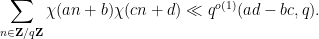
Now we prove (23), which is where we need nontrivial bounds on Kloosterman sums. Expanding out ${\mu f * 1}$ and using the triangle inequality, it suffices (for ${C}$ large enough) to show that

$\displaystyle \sum_{n: (n(n+2),W)=1; r|n(n+2)} (\sum_{d|n(n+2)} \chi(d) G_\sim( \frac{\log d}{\log x} )) \psi_x(n) \ll q^{O(1)} x^{0.99+o(1)}$

for all ${r < q^{1/2}}$ . By Fourier expansion of the ${r|n(n+2)}$ and ${(n(n+2),W)=1}$ constraints (retaining only the restriction that ${n}$ is odd), it suffices to show that

$\displaystyle \sum_{n \hbox{ odd}} (\sum_{d|n(n+2)} \chi(d) G_\sim( \frac{\log d}{\log x} )) \psi_x(n) e( kn/Wr )\ll q^{O(1)} x^{0.99+o(1)}$

for every ${k \in {\bf Z}/Wr{\bf Z}}$ .

Fix ${r,k}$ . If ${d|n(n+2)}$ for an odd ${n}$ , then we can uniquely factor ${d = d_1 d_2}$ such that ${d_1|n}$ , ${d_2|n+2}$ , and ${(d_1,d_2)=1}$ . It thus suffices to show that

$\displaystyle \sum_{d_1,d_2: (d_1,d_2)=1} \chi(d_1) \chi(d_2) G_\sim( \frac{\log d_1 + \log d_2}{\log x} )) \ \ \ \ \ (25)$

$\displaystyle \sum_{n \hbox{ odd}: d_1|n; d_2|n+2}\psi_x(n) e( kn/Wr)$

$\displaystyle \ll q^{O(1)} x^{0.99+o(1)}.$

Actually, we may delete the condition ${(d_1,d_2)=1}$ since this is implied by the constraints ${d_1|n, d_2|n+2}$ and ${n}$ odd.

We first dispose of the case when ${d_1}$ is large in the sense that ${d_1 \geq x^{0.51}}$ . Making the change of variables ${d_3 = n/d_1}$ , we may rewrite the left-hand side as

$\displaystyle \sum_{d_3,d_2} \chi(d_2) \sum_{n \hbox{ odd}: d_3|n; d_2|n+2} \chi( \frac{n}{d_3} ) G_\sim( \frac{\log n - \log d_3 + \log d_2}{\log x} )$

$\displaystyle \psi_x(n) e(kn/Wr).$

We can assume ${d_2}$ is coprime to ${q}$ and ${d_2,d_3}$ odd with ${d_3}$ coprime to ${d_2}$ and ${d_2,d_3 \ll x^{0.49}}$ , as the contribution of all other cases vanish. The constraints that ${n}$ is odd and ${d_3|n, d_2|n+2}$ then restricts ${n}$ to a single residue class modulo ${2 d_2 d_3}$ , with ${n/d_3}$ restricted to a single residue class modulo ${2 d_2}$ . We split this into ${Wr}$ residue classes modulo ${2Wd_2 r}$ to make the ${e(kn/Wr)}$ phase constant on each residue class. The modulus ${2Wd_2 r}$ is not divisible by ${q}$ , since ${d_2}$ is coprime to ${q}$ and ${r \leq \sqrt{q}}$ . As such, ${\chi(\frac{n}{d_3})}$ has mean zero on every consecutive ${q}$ elements in each residue class modulo ${2Wd_2 r}$ under consideration, and from summation by parts we then have

$\displaystyle \sum_{n \hbox{odd}: d_3|n; d_2|n+2} \chi( \frac{n}{d_3} ) G_\sim( \frac{\log n - \log d_3 + \log d_2}{\log x} ) \psi_x(n) e(kn/Wr)$

$\displaystyle \ll q Wr$

and hence the contribution of the ${d_1 \geq x^{0.51}}$ case to (25) is

$\displaystyle \ll \sum_{d_3,d_2 \ll x^{0.49}} q Wr \ll q^{O(1)} x^{0.98}$

which is acceptable.

It remains to control the contribution of the ${d_1 < x^{0.51}}$ case to (25). By the triangle inequality, it suffices to show that

$\displaystyle \sum_{d_2} \chi(d_2) G_\sim( \frac{\log d_1 + \log d_2}{\log x} )) \sum_{n \hbox{odd}: d_1|n; d_2|n+2}\psi_x(n) e(kn/Wr)$

$\displaystyle \ll q^{O(1)} x^{0.99+o(1)} / d_1$

for all ${d_1 < x^{0.51}}$ coprime to ${q}$ . We can of course restrict ${d_1,d_2}$ to be coprime to each other and to ${W}$ . Writing ${n+2 = d_2 (2m+1)}$ , the constraint ${d_1|n}$ is equivalent to

$\displaystyle m = \overline{d_2} - \overline{2} \hbox{ mod } d_1$

and so we can rewrite the left-hand side as

$\displaystyle \sum_{d_2: (d_1,d_2)=1} \chi(d_2) G_\sim( \frac{\log d_1 + \log d_2}{\log x} ))$

$\displaystyle \sum_{m = \overline{d_2} - \overline{2} \hbox{ mod } d_1} \psi_x(d_2 (2m+1)-2) e(k(d_2(2m+1))/Wr) e(-2k/Wr).$

By Fourier expansion, we can write ${\chi(d_2)}$ as a linear combination of ${e( l d_2 / q)}$ with bounded coefficients and ${(l,q)=1}$ , so it suffices to show that

$\displaystyle \sum_{d_2: (d_1,d_2)=1} e(ld_2/q) G_\sim( \frac{\log d_1 + \log d_2}{\log x} ))$

$\displaystyle \sum_{m = \overline{d_2} - \overline{2} \hbox{ mod } d_1} \psi_x(d_2 (2m+1)-2) e( 2kd_2 m / Wr )$

$\displaystyle \ll q^{O(1)} x^{0.99+o(1)} / d_1.$

Next, by Fourier expansion of the constraint ${m = \overline{d_2} - \overline{2} \hbox{ mod } d_1}$ , we write the left-hand side as

$\displaystyle \frac{1}{d_1} \sum_{h \in {\bf Z}/d_1 {\bf Z}} \sum_{d_2: (d_1 d_2)=1} e(ld_2/q) G_\sim( \frac{\log d_1 + \log d_2}{\log x} )) e( h(\overline{d_2} - \overline{2})/d_1)$

$\displaystyle \sum_m e(-hm/d_1) \psi_x(d_2 (2m+1)-2) e( 2kd_2 m / Wr ).$

From Poisson summation and the smoothness of ${\psi}$ , we see that the inner sum is ${O(x^{-100})}$ unless

$\displaystyle \| \frac{h}{d_1} - \frac{c}{Wr} \| \ll \frac{x^{0.01}d_2}{x} \ \ \ \ \ (26)$

for some integer ${c}$ , where ${\|\theta\|}$ denotes the distance from ${\theta}$ to the nearest integer. The contribution of the ${h}$ which do not satisfy this relation is easily seen to be acceptable. From the support of ${G_\sim}$ we see in particular that there are only ${O( r x^{0.03} )}$ remaining choices for ${h}$ . Thus it suffices by the triangle inequality to show that

$\displaystyle \sum_{d_2: (d_1 d_2)=1} e(ld_2/q) G_\sim( \frac{\log d_1 + \log d_2}{\log x} )) e( h\overline{d_2}/d_1)$

$\displaystyle \sum_m e(-hm/d_1) \psi_x(d_2 (2m+1)-2) e( 2kd_2 m / Wr )$

$\displaystyle \ll q^{O(1)} x^{0.95}$

for each ${h \in {\bf Z}/d_1{\bf Z}}$ of the form (26).

We rearrange the left-hand side as

$\displaystyle \sum_m e(-hm/d_1) \sum_{d_2: (d_1 d_2)=1} e(kd_2/q) G_\sim( \frac{\log d_1 + \log d_2}{\log x} )) e( h\overline{d_2}/d_1)$

$\displaystyle e( 2kd_2 m / Wr ) \psi_x(d_2 (2m+1)-2).$

Suppose first that ${h/d_1}$ is of the form ${c/Wr}$ for some integer ${c}$ . Then the phase ${d_2 \mapsto e(kd_2/q) e( h\overline{d_2}/d_1) e( 2kd_2 m / Wr )}$ is periodic with period ${Wqr}$ and has mean zero here (since ${Wr<q}$ ). From this, we can estimate the inner sum by ${O( Wqr )}$ ; since ${m}$ is restricted to be of size ${O( x / d_2 ) = O( x^{0.02} d_1 ) = O( x^{0.53} )}$ , this contribution is certainly acceptable. Thus we may assume that ${h/d_1}$ is not of the form ${c/Wr}$ . A similar argument works when ${d_1 \leq x^{0.4}}$ (say), so we may assume that ${d_1 \geq x^{0.4}}$ , so that ${d_2 \ll x^{0.6}}$ .

By (26), this forces the denominator of ${h/d_1}$ in lowest form to be ${\gg \frac{x}{x^{0.01} d_2 Wr} \gg q^{-O(1)} x^{0.39}}$ . By Lemma 2, we thus have

$\displaystyle \sum_{d_2 \in ({\bf Z}/d_1{\bf Z})^\times} e( a d_2/d_1) e( h\overline{d_2}/d_1) \ll x^{o(1)} d_2 ( q^{-O(1)} x^{0.39} )^{-1/4}$

$\displaystyle \ll q^{O(1)} x^{-0.09} d_2$

for any ${a}$ , so from Poisson summation we have

$\displaystyle \sum_{d_2: (d_1 d_2)=1} e(kd_2/q) G_\sim( \frac{\log d_1 + \log d_2}{\log x} )) e( h\overline{d_2}/d_1) e( 2kd_2 m / Wr )$

$\displaystyle \psi_x(d_2 (2m+1)-2) \ll q^{O(1)} x^{-0.07} \frac{x}{d_1};$

since ${m}$ is constrained to be ${O( x^{0.02} d_1 )}$ , the claim follows.

Finally, we prove (22), which is a routine sieve-theoretic calculation. We rewrite the left-hand side as

$\displaystyle \sum_{d,e} \chi(d) G_<(\frac{\log d}{\log x}) \mu(e) f(e) \sum_n 1_{n: (n(n+2),W)=1; [d,e] | n(n+2)} \psi_x(n).$

The summand vanishes unless ${d,e}$ are coprime to ${W}$ with ${d \ll x^{0.52}}$ and ${e \leq \sqrt{q}}$ . From Poisson summation one then has

$\displaystyle \sum_n 1_{m: (n(n+2),W)=1; [d,e] | n(n+2)} \psi_x(n) = \frac{1}{2} (\prod_{2 < p \leq w} (1-\frac{2}{p})) (\int_{\bf R} \psi) \frac{x \log^{-C} x 2^{\omega([d,e])}}{[d,e]}$

$\displaystyle + O( x^{-100} ).$

The error term is certainly negligible, so it suffices to show that

$\displaystyle (\prod_{2 < p \leq w} (1-\frac{2}{p})) \sum_{d,e: (de,W)=1} \chi(d) G_<(\frac{\log d}{\log x}) \mu(e) \psi(\frac{\log e}{\log q}) \frac{2^{\omega([d,e])}}{[d,e]}$

$\displaystyle \gg (1-o(1)) \log^{-2} x.$

We can control the left-hand side by Fourier analysis. Writing

$\displaystyle e^u G_<(u) = \int_{\bf R} g(t) e^{-itu}\ dt$

and

$\displaystyle e^u \psi(u) = \int_{\bf R} \Psi(t) e^{-itu}\ dt$

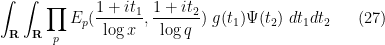
for some rapidly decreasing functions ${g,\Psi}$ , the left-hand side may be expressed as

$\displaystyle (\prod_{2 < p \leq w} (1-\frac{2}{p})) \int_{\bf R} \int_{\bf R} \sum_{d,e: (de,W)=1} \frac{\chi(d) \mu(e)2^{\omega([d,e])}}{[d,e] d^{\frac{1+it_1}{\log x}} e^{\frac{1+it_2}{\log q}}}\ g(t_1) \Psi(t_2)\ dt_1 dt_2$

which factors as

$\displaystyle \int_{\bf R} \int_{\bf R} \prod_p E_p( \frac{1+it_1}{\log x}, \frac{1+it_2}{\log q} ) \ g(t_1) \Psi(t_2)\ dt_1 dt_2 \ \ \ \ \ (27)$

where

$\displaystyle E_2(s_1,s_2) := 1$

$\displaystyle E_p(s_1,s_2) := 1 - \frac{2}{p}$

for ${p \leq w}$ , and

$\displaystyle E_p(s_1,s_2) := 1 - 2\frac{1}{p^{1+s_2}} + 2\sum_{j=1}^\infty \frac{\chi(p)^j}{p^{j(1+s_1)}} (1 - \frac{1}{p^{s_2}})$

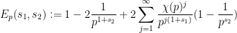
for ${p>w}$ . From Mertens’ theorem we have the crude bound

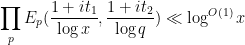$\displaystyle \prod_p E_p( \frac{1+it_1}{\log x}, \frac{1+it_2}{\log q} ) \ll \log^{O(1)} x$

which by the rapid decrease of ${g,\Psi}$ allows one to restrict to the range ${|t_1|, |t_2| \leq \sqrt{\log q}}$ with an error of ${o(\log^{-1} x)}$ . In particular, we now have ${s_1,s_2 = o(1)}$ .

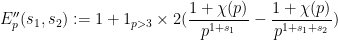
Recalling that

$\displaystyle \zeta(s) = \prod_p (1 - \frac{1}{p^s})^{-1}$

for ${\hbox{Re}(s)>1}$ , we can factor

$\displaystyle \prod_p E_p( s_1, s_2 ) = \frac{\zeta^2(1 + s_1+s_2)}{\zeta^2(1+s_1) \zeta^2(1+s_2)} \prod_p E'_p(s_1,s_2) E''_p(s_1,s_2)$

where

$\displaystyle E''_p(s_1,s_2) := 1 + 1_{p>3} \times 2 (\frac{1+\chi(p)}{p^{1+s_1}} - \frac{1+\chi(p)}{p^{1+s_1+s_2}})$

(the restriction ${p>3}$ being to prevent ${E''_p(s_1,s_2)}$ vanishing for ${p=2,3}$ and ${s_1,s_2}$ small) and one has

$\displaystyle E'_p(s_1,s_2) = 1 + O( \frac{1}{p^{2+o(1)}} )$

for ${s_1,s_2 = o(1)}$ , and

$\displaystyle E_2(0,0) = 2$

and

$\displaystyle E_p(0,0) = 1$

for odd ${p}$ . In particular, from the Cauchy integral formula we see that

$\displaystyle \prod_p E'_p(s_1,s_2) = 2 + o(1)$

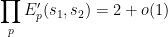for ${s_1,s_2 = o(1)}$ . Since we also have ${\zeta(1+s) = \frac{1+o(1)}{s}}$ in this region, we thus can write (27) as

$\displaystyle \int_{|t_1|, |t_2| \leq \sqrt{\log q}} (1+o(1)) \prod_p E''_p(s_1,s_2) \frac{(1+it_2)^2 (1+it_1)^2}{(1+it_2 + \frac{1+it_1}{C})^2 \log^2 x}$

$\displaystyle g(t_1) \Psi(t_2) dt_1 dt_2 + o(\log^{-2} x)$

and our task is now to show that

$\displaystyle \int_{|t_1|, |t_2| \leq \sqrt{\log q}} (1+o(1)) \prod_p E''_p(s_1,s_2) \frac{(1+it_2)^2 (1+it_1)^2}{(1+it_2 + \frac{1+it_1}{C})^2}$

$\displaystyle g(t_1) \Psi(t_2) dt_1 dt_2 \gg 1 - o(1).$

We have

$\displaystyle \log E''_p(s_1,s_2) = O(1/p)$

when ${s_1,s_2 = O(\frac{1}{\log p})}$ (even when ${s_1,s_2}$ have negative real part); since ${\log E''_p(0,0)=0}$ , we conclude from the Cauchy integral formula that

$\displaystyle \log E''_p(s_1,s_2) \ll (|s_1|+|s_2|) \frac{\log p}{p}$

when ${\log p \ll \frac{1}{|s_1|+|s_2|}}$ . For the remaining primes ${p}$ , we have

$\displaystyle \log E''_p(s_1,s_2) \ll \frac{1+\chi(p)}{p^{1+1/\log x}}$

when ${s_1 = \frac{1+it_1}{\log x}}$ and ${s_2 := \frac{1+it_2}{\log q}}$ . Summing in ${p}$ using Lemma 5 to handle those ${p}$ between ${q}$ and ${x}$ , and Mertens’ theorem and the trivial bound ${1+\chi(p)=O(1)}$ for all other ${p}$ , we conclude that

$\displaystyle \sum_p \log E''_p(s_1,s_2) \ll \log( 2+|s_1|+|s_2| )$

and thus

$\displaystyle \prod_p E''_p(s_1,s_2) \ll (2 + |s_1| + |s_2| )^{O(1)}.$

From this and the rapid decrease of ${g,\Psi}$ , we may restrict the range of ${t_1,t_2}$ even further to ${|t_1|, |t_2| \leq \omega(q)}$ for any ${\omega(q)}$ that goes to infinity arbitrarily slowly with ${q}$ . For sufficiently slow ${\omega}$ , the above estimates on ${\log E''_p(s_1,s_2)}$ and Lemma 5 (now used to handle those ${p}$ between ${q^\varepsilon}$ and ${x^{1/\varepsilon}}$ for some ${\varepsilon}$ going sufficiently slowly to zero) give

$\displaystyle \sum_p \log E''_p(s_1,s_2) = o(1)$

and so we are reduced to establishing that

$\displaystyle \int_{|t_1|, |t_2| \leq \omega(q)} (1+o(1)) \frac{(1+it_2)^2 (1+it_1)^2}{(1+it_2 + \frac{1+it_1}{C})^2}\ g(t_1) \Psi(t_2) dt_1 dt_2 \gg 1 - o(1).$

We may once again use the rapid decrease of ${g,\Psi}$ to remove the ${o(1)}$ prefactor as well as the restrictions ${|t_1|, |t_2| \leq \omega(q)}$ , and reduce to showing that

$\displaystyle \int_{\bf R} \int_{\bf R} \frac{(1+it_2)^2 (1+it_1)^2}{(1+it_2 + \frac{1+it_1}{C})^2}\ g(t_1) \Psi(t_2) dt_1 dt_2 \gg 1 - o(1).$

For ${C}$ large enough, it will suffice to show that

$\displaystyle \int_{\bf R} \int_{\bf R} (1+it_1)^2\ g(t_1) \Psi(t_2) dt_1 dt_2 \gg 1$

with the implied constant independent of ${C}$ . But the left-hand side evaluates to ${G''_<(0) \psi(0) = 2 \psi(0)}$ , and the claim follows.

76 comments

Comments feed for this article

26 August, 2015 at 10:59 pm

Anonymous

Is there any known probabilistic argument for the existence/ nonexistence of Siegel zeros?

27 August, 2015 at 8:08 am

Terence Tao

Probabilistic arguments (in particular, the Mobius pseudorandomness principle, discussed in this previous post) suggest that the generalised Riemann Hypothesis (GRH) is true, which can be viewed as the polar opposite of having a Siegel zero (certainly the two statements are incompatible). As such, the Siegel zero problem is really quite tantalising; it is the strongest surviving alternative to the conjectural picture we have about the distribution of the primes, and eliminating it would be viewed as a significant advance towards the GRH (although there would still be a lot further to go to finish that off entirely). (Historically, there were GRH alternatives that were even stronger than the Siegel zero, such as the “tenth discriminant”, but these at least have been eliminated, though not without quite a bit of effort.)

4 September, 2015 at 4:31 am

Sergei

It is an interesting idea to use an unsquared Selberg sieve.
In fact, on the generalized Elliott-Halberstam conjecture
an unsquared Selberg sieve weight does correlate with the MÃ¶bius function,
and this can be used to deduce the twin prime conjecture from
the generalized Elliott-Halberstam conjecture.

The idea is to use the unsquared sieve weight

$\displaystyle R(\lambda) := \lambda - \lambda ( 1_{{\mathcal P}_1\cup{\mathcal P}_3\cup\dots } (n+h_1) 1_{{\mathcal P}_2\cup{\mathcal P}_4\cup\dots } (n+h_2) + 1_{{\mathcal P}_2\cup{\mathcal P}_4\cup\dots } (n+h_1) 1_{{\mathcal P}_1\cup{\mathcal P}_3\cup\dots }(n+h_2) ),$

where ${1_{S}(n)}$ is the indicator function of $S$ and ${{\mathcal P}_r}$ is the set of squarefree integers
which have exactly $r$ prime factors.

Now assume the generalized Elliott-Halberstam conjecture, and let ${0 < c < 1}$ be a real number to be chosen later.
Define the function ${(f)_{{+}}}$ to be $f$ when $f$ is positive, and $0$ otherwise.

Take

$\displaystyle f(x,y) := (c-x)_{{+}}(c-y)_{{+}}.$

Consider the weighted expression

$\displaystyle \sum_{N\leq n\leq 2N,\ n\equiv b\ (W)} R(\lambda_{f}(n))$

$\displaystyle \times (\theta(n+h_1)+\theta(n+h_2)-\log 3N)$

where

$\displaystyle \lambda_{f}(n) := \sum_{d_1 | (n+h_1),\ d_2 | (n+h_2)}\mu(d_1)\mu(d_2) f(\frac{\log d_1}{\log N},\frac{\log d_2}{\log N}).$

Using Theorems 3.5, 3.6 of Polymath8b, it can be shown that

$\displaystyle \sum_{N\leq n\leq 2N,\ n\equiv b\ (W)}\lambda_{f}(n)$

$\displaystyle \times (\theta(n+h_1)+\theta(n+h_2)-\log 3N)$

$\displaystyle = (I+o(1))\frac{WN}{\varphi^2(W)\log N}$

for ${I > 0}$ fixed if $c$ is close enough to $1$ .
(note that integers for which $n+h_1$ or $n+h_2$ has a small prime factor give negligible contribution).

According to Chapter 16 of Friedlander-Iwaniec, if there are no pairs $n+h_1$ prime, $n+h_2$ prime, then

$\displaystyle 1_{{\mathcal P}_1\cup{\mathcal P}_3\cup\dots }(n+h_1)1_{{\mathcal P}_2\cup{\mathcal P}_4\cup\dots }(n+h_2) + 1_{{\mathcal P}_2\cup{\mathcal P}_4\cup\dots }(n+h_1)1_{{\mathcal P}_1\cup{\mathcal P}_3\cup\dots }(n+h_2)$

has a completely determined distribution function, so we can compute that

$\displaystyle \sum_{N\leq n\leq 2N,\ n\equiv b\ (W)} -\lambda_{f}(n)$

$\displaystyle \times (1_{{\mathcal P}_1\cup{\mathcal P}_3\cup\dots }(n+h_1)1_{{\mathcal P}_2\cup{\mathcal P}_4\cup\dots }(n+h_2)+1_{{\mathcal P}_2\cup{\mathcal P}_4\cup\dots }(n+h_1)1_{{\mathcal P}_1\cup{\mathcal P}_3\cup\dots }(n+h_2))$

$\displaystyle \times (\theta(n+h_1)+\theta(n+h_2)-\log 3N)$

$\displaystyle \geq (-\varepsilon(c)+o(1))\frac{WN}{\varphi^2(W)\log N},$

where ${\varepsilon(c)\to 0}$ as ${c\to 1}$ .

Choosing $c$ close enough to $1$ ,
we get ${I-\varepsilon(c) > 0}$ and hence

$\displaystyle 1_{{\mathcal P}_1\cup{\mathcal P}_3\cup\dots }(n+h_1)1_{{\mathcal P}_1\cup{\mathcal P}_3\cup\dots }(n+h_2)+1_{{\mathcal P}_2\cup{\mathcal P}_4\cup\dots }(n+h_1)1_{{\mathcal P}_2\cup{\mathcal P}_4\cup\dots }(n+h_2)$

has a nonzero distribution function, and again by Chapter 16 of Friedlander-Iwaniec
it follows that

$\displaystyle 1_{{\mathcal P}_1}(n+h_1)1_{{\mathcal P}_1}(n+h_2)$

has a nonzero distribution function.

4 September, 2015 at 7:22 am

Terence Tao

I think that if you do the calculations carefully (in particular paying attention to the main terms that are not directly treatable by GEH, coming from convolutions in which one factor is supported very close to the origin or which otherwise fails to obey a Siegel-Walfisz condition), you will find that $\varepsilon(c)$ converges to I, not to 0, as $c \to 1$ .

For the twin prime problem, even with GEH, one has the parity problem scenario in which $\lambda(n) = - \lambda(n+2)$ for all (or almost all) $n$ for which $n,n+2$ are almost prime (here $\lambda$ is the Liouville function, not the sieve weight). In this scenario there are essentially no twin primes (since for such primes $p$ one has $\lambda(p)=\lambda(p+2)=-1$ ), and your weight $1_{{\mathcal P}_1 \cup \dots}(n) 1_{{\mathcal P}_2 \cup \dots}(n+2) + 1_{{\mathcal P}_2 \cup \dots}(n) 1_{{\mathcal P}_1 \cup \dots}(n+2)$ is essentially equal to 1. This scenario is consistent with GEH (assuming Mobius pseudorandomness) and with all other known inputs available to sieve theory, including those in Friedlander-Iwaniec. From the work of Bomberi we know that (on EH) this scenario is essentially the only scenario in which we have essentially no twin primes.

Personally, I advise against spending too much time on trying to attack the twin prime conjecture under hypotheses such as GEH unless you can pinpoint the precise input you are using (or hope to use) which breaks the parity barrier by being incompatible (at least from a heuristic, moral, or conjectural standpoint) with the $\lambda(n)=-\lambda(n+2)$ scenario. (For instance, in the current blog post it is Lemma 3 which is providing the incompatibility, because the Siegel zero forces $\lambda$ to behave like $\chi$ on almost primes, and Lemma 3 (plus some sieve theory) precludes the $\chi(n) = - \chi(n+2)$ scenario on such almost primes.)

4 September, 2015 at 10:42 pm

Sergei

Yes, the weight $1_{{\mathcal P}_1 \cup \dots}(n) 1_{{\mathcal P}_2 \cup \dots}(n+2) + 1_{{\mathcal P}_2 \cup \dots}(n) 1_{{\mathcal P}_1 \cup \dots}(n+2)$ is essentially equal to $1$ in this unique scenario, but in this scenario the unsquared weight $\lambda_{f}(n)$ is essentially equal to $0$ on the primes $p$ for which $\lambda(p)=-\lambda(p+2)$ . It is different from the weight in the squared Selberg sieve, which is NOT essentially equal to $0$ in this case?

4 September, 2015 at 11:05 pm

Terence Tao

Actually, I don’t think $\lambda_f$ is all that small on those primes $p$ for which $\lambda(p) = - \lambda(p+2)$ (note that $p+2$ will likely have some prime factors less than $x^{1-c}$ ; this is a subtlety that also shows up in Bombieri’s analysis… one can insert a further sieve to eliminate extremely small prime factors, but not factors of size near $x^{1-c}$ unless one damps the function $f$ to a higher order near $1-c$ ). Indeed, Mobius pseudorandomness heuristics predict that $\lambda_f(n)$ will be asymptotically orthogonal to $\lambda(n+2)$ (whether one restricts $n$ to be prime or not) and so the value of $\lambda(n+2)$ should have essentially no influence on the behaviour of $\lambda_f(n)$ .

To repeat my previous comment, the parity problem is not an obstacle to be taken lightly. If you haven’t identified a precise input in your argument which is explicitly getting around the parity barrier (basically, one needs to somehow control a sum of an expression that has a nontrivial correlation with $\lambda(n) \lambda(n+2)$ , which none of the standard sieve weights do even when weighted by $\theta(n)$ or $\theta(n+2)$ ), the chances are overwhelmingly likely that there is going to be an error in your analysis.

5 September, 2015 at 10:59 pm

Sergei

I absolutely agree that the parity barrier is a very serious problem. It is not entirely clear where is the moral difference between the 2-dimensional weights

$\displaystyle \lambda_{f_1}(n) := \sum_{d_1 | n,\ d_2 | (n+2)}\mu(d_1)\mu(d_2) f_1(\frac{\log d_1}{\log N},\frac{\log d_2}{\log N})$

where

$\displaystyle f_1(x,y) := (c-x)_{{+}}(c-y)_{{+}}$

and

$\displaystyle \lambda_{f_2}(n)^2 := \left( \sum_{d_1 | n,\ d_2 | (n+2)}\mu(d_1)\mu(d_2) f_2(\frac{\log d_1}{\log N},\frac{\log d_2}{\log N})\right)^2$

where

$\displaystyle f_2(x,y) := (c/2-x)_{{+}}(c/2-y)_{{+}}.$

I don’t quite see how $\lambda_{f_1}(p)$ could be large when $p+2$ has one (say) prime factor less than $x^{1-c}$ . But it is clear that $\lambda_{f_2}(p)^2$ could be large when $p+2$ has one prime factor less than $x^{1-c/2}$ .

6 September, 2015 at 10:02 am

Terence Tao

Note that $\lambda_{f_1}(n)$ factors as $\alpha(n) \alpha(n+2)$ , where $\alpha(n) := \sum_{d|n} (c - \frac{\log d}{\log N})_+ \mu(d)$ . Next, since

$\sum_{d|n} (c - \frac{\log d}{\log N}) \mu(d) = \frac{1}{\log N} \Lambda(n)$

we can write

$\alpha(n) = \frac{1}{\log N} \Lambda(n) + \sum_{d|n} (\frac{\log d}{\log N} - c)_+ \mu(d)$

which on replacing $d$ by $n/d$ is essentially (assuming $n$ squarefree and close to $N$ for simplicity)

$\alpha(n) \approx \frac{1}{\log N} \Lambda(n) + \lambda(n) \sum_{d|n} ((1-c) - \frac{\log d}{\log N})_+ \mu(d).$

If $1-c = \varepsilon$ , the latter term is roughly speaking like $\varepsilon \lambda(n)$ restricted to those numbers that are $N^\varepsilon$ -rough (have no prime factors much smaller than $N^\varepsilon$ ). This latter set of numbers is larger than the set of primes by a factor of about $1/\varepsilon$ . So, while $\alpha$ is of size about 1 on primes, it is also of size about $\varepsilon$ on a set of size about $1/\varepsilon$ larger than the primes, and the net contribution of this set is of equal strength (in an L^1 sense) to the contribution on primes. (It may be small in an $L^\infty$ sense, but it is the $L^1$ size which is the most relevant for these computations.) For instance, it is an instructive exercise to compute $\sum_{n \leq N} \alpha(n) \lambda(n)$ and find out that this is rather small (as is predicted from the Mobius pseudorandomness principle – $\alpha$ has to give an equal weight to numbers with an odd number of prime factors, and numbers with an even number of prime factors), even though the contribution coming from the primes (or even from all of the numbers with all prime factors larger than $N^{1-c}$ ) is quite large.

Returning to $\lambda_{f_1}(n) = \alpha(n) \alpha(n+2)$ , we now see that $\lambda_{f_1}(p)$ can be somewhat large (of size about $\varepsilon$ ) when the smallest prime factor of $p+2$ is comparable to $N^{\varepsilon}$ , and the contribution of this case to the $\varepsilon(c)$ in your original argument is of about the same size as the contribution of the case when $p+2$ is prime, which I believe will ultimately lead to $\varepsilon(c)$ converging to I rather than to 0 as I said in my first comment (this is the only possible limiting value for $\varepsilon(c)$ which is compatible with the Mobius pseudorandomness principle). In any event, it’s probably a good idea for you to work out the computation of $\varepsilon(c)$ in full detail.

—

By the way, here is a more explicit way to think about the parity obstruction for twin primes which may help you appreciate why the inputs you are using are not strong enough to give the conclusion you wish to obtain. Sieve theory relies on inputs that can take the form of upper or lower bounds on sums of arithmetic functions, e.g.

$\sum_n f(n) = X + O(E)$

$\sum_n f(n) \geq X_- - O(E)$

$\sum_n f(n) \leq X_+ + O(E)$ ,

(for some main terms $X, X_+, X_-$ and error magnitude $E$ , and various arithmetic functions $f$ , which may for instance be the restriction of some other arithmetic function, e.g. $\Lambda(n)$ or $\Lambda(n+2)$ , to a residue class $a\ (q)$ ) or on averaged bounds such as Elliott-Halberstam type bounds

$\sum_{q \leq Q} \sup_{(a,q)=1} |\sum_{n=a\ (q)} f(n) - X_q| \ll E.$

Sieve theory also takes as input pointwise inequalities

$f(n) \leq g(n)$

between arithmetic functions (e.g. the trivial bounds $\Lambda(n), \Lambda(n+2) \geq 0$ ).

The whole game of sieve theory is to try to cleverly take linear combinations of these inputs, weighted by suitable sieves, to ultimately deduce something like

$\sum_{p \leq N: p+2 \hbox{ prime}} 1 \geq Y - O(E)\quad (1)$

or perhaps

$\sum_{N \leq n \leq 2N} (\theta(n)+\theta(n+2)-\log 3N) \geq Y - O(E)\quad (2)$

where the main term $Y$ is significantly larger than the error term $E$ .

Call an estimate parity-insensitive if it is conjectured that the estimate is essentially unchanged after weighting the natural numbers $n$ by the weight $(1 - \lambda(n)\lambda(n+2))$ . For instance, Elliott-Halberstam type bounds on $\sum_{n=a\ (q)} \Lambda(n)$ are conjectured (by the Mobius pseudorandomness heuristic) to also hold for the weighted sum $\sum_{n=a\ (q)} \Lambda(n) (1 - \lambda(n) \lambda(n+2))$ ; similarly if $\Lambda(n)$ is replaced by $\Lambda(n+2)$ . Clearly any pointwise bound is also parity-insensitive since the weight $1 -\lambda(n)\lambda(n+2)$ is non-negative. In fact all of the standard inputs to sieve theory (including GEH) are conjectured to be parity-insensitive. On the other hand, bounds such as (1) or (2) are parity-sensitive (and the bounds you claim would also be parity sensitive if $\varepsilon(c)$ converged to any value other than I), because the weight $1 - \lambda(n) \lambda(n+2)$ vanishes on twin primes. It is also clear that taking linear combinations of parity-insensitive inequalities weighted by sieve weights can only ever yield more parity-insensitive inequalities, no matter how cleverly one chooses the sieve weights and the linear combinations. As such, it is not possible to produce twin primes by sieve theoretic arguments, unless one uses an input that is parity sensitive, or if one is operating under a hypothesis (such as a Siegel zero hypothesis) that is incompatible with the Mobius pseudorandomness heuristic. If you are unable to identify the precise parity sensitive input or pseudorandomness-violating hypothesis in your argument, this is a very strong signal that your argument is not correct.

6 September, 2015 at 11:10 pm

Sergei

Thanks for this! Very enlightening.

7 September, 2015 at 5:15 am

Sergei

Is it right that it is unclear what happens with the asymptotic for $\lambda_{f_1}(n)$ in the intermediate regime $c=1-o(1)$ for various $o(1)$ going to $0$ as $N \to \infty$ ?

7 September, 2015 at 8:19 am

Terence Tao

Depends on what you are trying to compute. A plain sum such as $\sum_{n \leq x} \lambda_{f_1}(n)$ should still be computable because the constant function $1$ is extremely well distributed in arithmetic progressions. However a sum such as $\sum_{n \leq x} \lambda_{f_1}(n) \theta(n+2)$ becomes very tricky, it involves understanding the distribution of $\theta(n+2)$ in arithmetic progressions of spacing up to $x^{1-c}$ and it is known that the Elliott-Halberstam conjecture breaks down for $c=1-o(1)$ sufficiently close to 1, see the work of Friedlander and Granville. It may still be possible to use a strong version of pseudorandomness hypotheses though (e.g. Montgomery’s conjecture on the error term in the prime number theorem in arithmetic progressions) to predict what happens. Of course in the limit $c=1$ , $\lambda_{f_1}$ is essentially the von Mangoldt function, which is sensitive to $\lambda(n)$ in contrast to the $c < 1 - \varepsilon$ cases, so there must be some transition behaviour at some point.

27 August, 2015 at 8:08 am

Will

Yes, the heuristic that the primes are distributed randomly (e.g. the Cramer model) suggests that the error term for the prime number theorem in arithmetic progressions is $O(n^{1/2+ \epsilon})$ , which implies no Siegel zeros.

27 August, 2015 at 10:24 am

David Speyer

Minor suggestion: Friedlander and Iwaniec is available freely and legally online http://www.ams.org/notices/200907/rtx090700817p.pdf , but your link requires MathSciNet access. You might want to switch to the free one.

[Link changed, thanks – T.]

27 August, 2015 at 11:13 am

David Speyer

By the way, I’d enjoy a blogpost laying out what the alternative “ghostly” world looks like. I’ve picked it up in bits and pieces from your posts on the parity problem and other sources, but it would be interesting to see it all in one place, laid out as a consistent alternative.

28 August, 2015 at 8:51 am

meditationatae

I find it very stimulating that you write about this “unlikely” “alternate universe”. I can recognize terminology (e.g. “damping” ) used in sieve theory, that is also common in electronic filter terminology (signal processing). Is this semblance of an analogy between filters and sieves worthy of some consideration by students or non-specialists of analytic number theory?

31 August, 2015 at 3:05 am

Anonymous

It is interesting to observe that the (hypothetical) asymptotic orthogonality of the Mobius function $\mu$ to all “structured” functions does not contradict the fact that $\mu$ has bounded algorithmic complexity.

31 August, 2015 at 5:27 am

meditationatae

It was my first encounter with Heath-Brown’s theorem. I’d like to know if there are heuristics or other things that give hope to analytic number theorists concerning which of (a) Twin Prime Conjecture, or (b) “No Siegel zeros”, “should” be the least difficult to prove?

26 March, 2023 at 5:26 am

Rather than focusing only on Siegel zeros, i think it would be interesting to investigate the consequences of the existence of any infinite sequence of non-real zeros whose real parts converge to 1. Such zeros actually seem to exist. Kindly see:

https://figshare.com/articles/preprint/Untitled_Item/14776146

26 March, 2023 at 8:06 am

Anonymous

same nonsense as before (same issues – forgetting dependencies)

26 March, 2023 at 10:21 am

Saying words like “nonsense” doesn’t make your comment any stronger or sensible. What exactly are the dependencies are you talking about ? Be explicitly clear.

26 March, 2023 at 10:47 am

Walfisz

@Anonymous, you’re probably referring to the implicit constant in (4) being dependent on epsilon, so that it may tend to infinity as epsilon tends to 0. However, that only becomes relevant if the author does let epsilon tend to 0.

Haven’t carefully checked other details, but the issue, if there is one, is definitely not on the the dependencies.

In short, you’re the one saying nonsense here.

27 March, 2023 at 10:32 am

Anonymous

the flaw has been detailed on MJR (when you truncate a convergent Dirichlet series at some fixed $x$ the remainder depends on both $s$ and $x$ and while it is true that for $s$ FIXED, the remainder goes to 0 when x to infinity, it is not true that happens uniformly in s so in particular for fixed x the remainder can be quite large when Im s is much larger – an easy example is t^(1/2)/x which goes to zero for fixed t when x goes to infinity but its integral in t is bigger than 1 as long as t is larger than x – this is essentially what happens in the Dirichlet case when uniform remainders are available precisely for x >> t= Im s only

29 March, 2023 at 9:52 pm

Okay thanks, but the crux of the argument here, is not the estimate of the remainder term. Rather, it’s the summation in (1), which, if Theta_{\chi} <1, creates a generalised Dirichlet eta function in the integrand.

In the calculations, we can actually work with the exact definition of E(x) = E(x, s, \overline{\chi}).

29 March, 2023 at 11:28 pm

**Definitions.** Let: $\mu$ be the Mobius function, $\chi$ be a primitive Dirichlet character of modulus $q$ and $\Theta_{\chi} \in [\frac{1}{2}, 1]$ be the supremum of the real parts of the zeros of $L(s, \chi)$ . Define $M(x, \chi)=\sum_{n \leq x} \mu(n)\chi(n)$ and $\sigma=\Re(s)$ . Let $T \in \mathbb{R}_{\geq 1}.$

**Theorem 1.** *One has $\Theta_{\chi}=1$ for every $\chi$ .*

**PROOF.** Suppose that $\Theta_{\chi}<1$ for some $\chi$ , and let $0<\varepsilon \Theta_\chi$ , it follows by Perron’s formula (Theorem 5.2 of
Montgomery-Vaughan (M.V.)) that
$

latex \displaystyle $/p>

Multiplying both sides of (1) by $\frac{(-1)^{n-1}\overline{\chi}(n)}{n}$ and summing from $n=1$ to $n=x$ gives

$ latex \displaystyle $

Since $\sum_{n=1}^{\infty} (-1)^{n-1}\overline{\chi}(n)n^{-z} =(1-2^{1-z})L(z, \overline{\chi})$ for $\Re(z) >0$, note that at $\sigma=\Theta_{\chi}+\varepsilon < 1$ , we have

$
latex \displaystyle $
where for $\Re(1-z)>0$ we have $E(x, z, \overline{\chi})=-\sum_{n>x} (-1)^{n-1}\overline{\chi}(n)n^{z-1} \ll 1$ uniformly for $x \geq 1$ . Inserting (3) into the right-hand side of (2) gives

$
latex \displaystyle
$/p>

Let $a_{\chi}=0$ if $\chi(-1)=1$ , and $a_{\chi}=1$ if $\chi(-1)=-1$ . Let $\rho_m$ be a zero of $L(s, \chi)$ of order $m$ , where $0<\Re(\rho_m)1$ . Similarly, the integrand of the second integral has: simple poles at $s=-2k-a_{\chi}$ with residue $h(k):=-\frac{E(x, -2k-a_{\chi})}{2k+a_{\chi}}$ , poles of order $m$ at $s=\rho_{m}$ with residue $R(\rho_{m}, x)=\frac{1}{(m-1)!}\frac{d^{m-1}}{ds^{m-1}}\Big(\frac{(s-\rho_m)^m E(x, s, \overline{\chi})}{sL(s, \chi)}\Big)\Big|_{s=\rho_m} 1$ . Let $y \in \mathbb{R}_{<0}$ be a non-integer, so that $L(y, \chi) \neq 0$ . For $\sigma <0$ and $s \neq -2k-a_{\chi}$ , note that $\Big|\frac{L(1-s, \overline{\chi})}{L(s, \overline{\chi})}\Big| \ll |s|^{-1/2}$ [M.V., pp. 330 and 334] and $L(1-s, \overline{\chi}) \sim 1$ hence $\lim_{y \rightarrow -\infty} \int_{y-iT}^{y + iT} \frac{(1-2^s)L(1-s, \overline{\chi})}{sL(s, \chi)} \mathrm{d}s = 0 = \lim_{y \rightarrow -\infty} \int_{y - iT }^{y + iT} \frac{E(x, s, \overline{\chi})}{sL(s, \chi)} \mathrm{d}s$ . Thus by shifting the line of integration in (4) to $(-\infty - iT, -\infty + iT)$ and applying the residue theorem, we obtain

$
latex \displaystyle
f(x)&=\sum_{k=b_{\chi}}^{\infty} (g(k) + h(k)) + \sum_{|\Im(\rho_m)| \leq T} R(\rho_{m}, x) + \frac{E(x, 0, \overline{\chi})}{L(0,\chi)} + O(x^{1+\varepsilon}/T) \tag{5} \\
&= -\sum_{k=b_\chi}^{\infty}\Bigg( \frac{(1-2^{-2k-a_{\chi}})L(2k+1+a_{\chi}, \overline{\chi})}{2k+a_{\chi}} + \frac{E(x, -2k-a_{\chi})}{2k+a_{\chi}} \Bigg) + \sum_{|\Im(\rho_m)| \leq T} R(\rho_{m}, x) + O\Big(1 + \frac{x^{1+\varepsilon}}{T} \Big). \tag{6}
>$

Since $\latex R(\rho_m, x) x}\frac{(-1)^{n-1}\overline{\chi}(n)}{n^{2k+a_{\chi}+1}} \ll \sum_{n > x} n^{-2} \ll x^{-1}$ for every non-negative integer $k$ . Hence the summands of the first sum are $> \frac{1}{3k}$ for any fixed large enough $x$ and all $k \geq k_0$ , thus the sum diverges as claimed. But we now have a contradiction, since $|f(x)|=|\sum_{n \leq x} \frac{(-1)^{n-1}M(n, \chi)\overline{\chi}(n)}{n}| q$ .

30 March, 2023 at 12:21 am

Apparently, therearesomeLaTex typos in the previous comment. So, you may see the actual paper:

https://figshare.com/articles/preprint/Untitled_Item/14776146

30 April, 2023 at 2:19 am

Anonymous

@TK, it really seems you’ve actually disproved the RH. Have you submitted this anywhere yet?

30 April, 2023 at 10:19 am

Anonymous

Tk talking to TK – the wonders of sock pupetry

30 April, 2023 at 1:26 pm

Anonymous

TK haters, you should be ashamed of yourselves for hating on someone with such talent and passion as TK.

1 May, 2023 at 3:42 am

@Anonymous: I submitted the paper to the Annals of Mathematics, but they’re yet to acknowledge receipt of the submission. However, I should mention that all the journals I submitted to before the Annals, returned the paper without any review comments. Some of the editors said that before submitting, I should discuss my work with some “experts”. But when I contact the “experts”, most of them suggest I send the work to some journal since it’s their job to review. I have therefore decided to post the work here, since the main result of the paper could be of relevance to this particular post.

1 May, 2023 at 11:28 am

Anonymous

Fun discussion between TK & David Farmer about this paper on MathOverflow:

https://mathoverflow.net/questions/445426/reference-request-for-pi-sum-im-rho-leq-t-n-rho-t-lambdan-o

Not sure it’s the David Farmer from AIM, though, given the ridiculously flawed comments he is posting.

1 May, 2023 at 3:56 pm

Anonymous

As usual, when someone took the time to show your errors, you reply with insults and nitpicking without actually thinking through what they say so do not be surprised that the number of people willing to engage is growing smaller and smaller;

1 May, 2023 at 10:36 pm

Which insults?? Didn’t I objectively reply in the MO post with factual mathematical comments which you have obviously chosen to ignore to suit your narrative?

The claim that David Farmer made in the now deleted MO post, is that for $\gamma \in [T, 2T], f(T, \rho)=\sum_{n \leq \log T} (-1)^{n-1} n^{\rho-1}$ doesn’t converge as $T \rightarow \infty$ , but tbis is not rrue at all. Inded, here is an elementary argument why $f(T, \rho)$ converges (to $(1-2^{\rho})\zeta(1-\rho)=0$ ) as $T$ tends to infinity.

Let $a_n = a_{n, \rho} = n^{\rho-1}$ and $b_n = (-1)^{n-1}$ . Then $ latex a_n$ decreases monotonically to 0 as $n$ tends to infinity, and

$ latex |\sum_{n \leq log T} b_n| \leq 1$

for all $T > e$ . Thus by mimicking the proof of the Dirichlet convergence test:

https://en.m.wikipedia.org/wiki/Dirichlet%27s_test

one deduces that $f(T, \rho)$ indeed converges (to $(1-2^{\rho})zeta(1-\rho)=0$ ) as $T$ tends to infinity. In particular, notice that this argument is independent of how large $|\rho|$ is.

1 May, 2023 at 10:55 pm

Walfisz

@Anonymous, please don’t impose your fallacious claims on TK. It’s a fact that $f(T, \rho) =\sum_{n \leq \log T} (-1)^{n-1}n^{\rho-1}$ converges as $T \rightarrow \infty$ , even if $|\rho| \approx T$ .

2 May, 2023 at 2:05 pm

Anonymous

when the experts point out to you why you are wrong, it is a good idea to at least consider they may have a point; after all you have been provably shown to be wrong by the same experts you have been disparaging for 100 times or more and the same thing is here, confusion between uniform and nonuniform bounds; nothing to do with analytic number theory, just basic analysis

2 May, 2023 at 2:29 pm

@David Farmer (commenting as “anonymous”, please vomment with your real name like I’m doing, as you informed me via email that you’re the most recent poster. Firstly, let it be known the public that you claimed via email yesterday that if the function $f(T, \rho)$ (which we can simply write as $f(T)$ since $\rho$ is a function of $T$ via $\gamma$ ) converges to 0 as $T$ tends to $\infty$ , then $f(T)$ can be close to $1$ for infinitely many $T$ . You and I both know that you uttered this statement, and I had to endure the trouble of explaining to you why it’s elementarily wrong even by the standards of first year undergrad calculus. It’s quite funny that you’re here now calling yourself an “expert”, despite claims such as this. This is the very reason why it’s difficult for you to understand why $f(T, \rho)$ converges as $T$ tends to $\infty$ . Next time, please comment with yout real name, David Farmer.

2 May, 2023 at 2:56 pm

John

For the benefit of some of us who didn’t see the now deleted MathOverflow post, can the constrictive critics please kindly point to us what exactly are you claiming to be the flaw? Surely, $f(T, \rho):=\sum_{n \leq \log T} (-1)^{n-1}n^{\rho-1}$ does converge independently of the magnitude of $|\rho|$ as $T \rightarrow \infty,$ since $f(T, \rho) = (1-2^{\rho})\zeta(\rho)- \sum_{n > \log T} (-1)^{n-1}n^{\rho-1}=-\sum_{n > \log T} (-1)^{n-1} n^{\rho-1}$ for all $T$.

2 May, 2023 at 5:35 pm

Alvarez

@Anonymous, which uniform/non uniform bounds are you talking about? I seem not to see any issue with uniformity.

3 May, 2023 at 4:58 am

Anonymous

The paper got debunked for (it’s number 100 or so after all and pretty much every time we heard the same combination of insults and assured statements that now this time is surely, utterly and of course 100% right) and no number of sock puppets make it correct. The MO thread (put as usual under false pretenses) and comments clearly showed it; talking from thin air about arbitrary stuff doesn’t change it.

3 May, 2023 at 6:23 am

John

@Anonymous, seems you have no valid mathematic criticism against the paper, except trash-talking against it and referring to previous versions. You have been asked to pinpoint the exact flaw in the current two page version, but you’re still beating around the bush. Not to mention how your tone sounds extremely bitter, lol.

3 May, 2023 at 6:38 am

Alvarez

@Anonymous, it’s funny that you keep referring to the now non-existent MO post that some of is didn’t come across. We’re asking you again for the second time: what exactly are you claiming to be the flaw? Otherwise stop speaking nonsense against someone who is working hard to actually make a meaningful contribution to mathematics.

4 May, 2023 at 7:44 am

The “issue” that was raised in the MathOverflow post is that, if $|\rho| > T$ , then $f(T, \rho)$ may not converge to $0$ as $T \rightarrow \infty$ . However, this is not true.

Indeed, fix $\sigma=\Re(s)T$ . Therefore, taking $s=\rho$ where $|\rho|$ yields $\lim_{T \rightarrow \infty} f(T, \rho)=(1-2^{\rho})\zeta(1-\rho)=0$ even if $|\rho|>T$ , as claimed. For the sake of completeness, I have added these details into the paper.

4 May, 2023 at 8:58 am

There are some LaTex typos in the above comment as I’m not used to MathJax. But you can see the revised version of Figshare in which I added the said details for explaining why $\lim_{T \rightarrow \infty} f(T, \rho)=0$ .

4 May, 2023 at 8:57 am

Anonymous

Good you put in details as they easily show how absurd your claim is since you take the limit of T to infinity and then claim that |\rho| >T; again same same (uniform vs pointwise), so nothing new; all debunked for the 100th time – looking forward to next try, though hopefully not too soon as it gets boring seeing same mistakes over and over

4 May, 2023 at 9:32 am

Peter

@Anonymous, why is it absurd that $|\rho|>T$ ? By the way, your choice of words should be more respectful. Your points do not become any stronger by trash-talking against the other person.

4 May, 2023 at 7:07 pm

Alvarez

@Anonymous, it’s so annoying how you’re so arrogant and disrespectful, yet completely ignorant. And, how did your flawed comment get 10 upvotes almost instantly? Using a VPN to upvote your nonsense?

4 May, 2023 at 11:29 am

Walfisz

@Anonymous, don’t be too desperate to debunk a paper without carefully reading and understanding what is written. Equation (10) is clearly uniform in $T \geq T_0$ . The author then later takes $|\rho|>T$ because that’s what’s relevant for the rest of the argument.

5 May, 2023 at 4:54 pm

Anonymous

Actually, there is a paper by Littlewood and Hardy whose methods can be easily adapted to show the divergence (when $T \to \infty$) of the sum $f(\rho(T), T)$ when $\rho(T) =\sigma +it, \sigma \le 1/2$ and $t$ around $T$ as D. Farmer mentioned on MO; the careless notation which doesn’t make it clear that the $\rho$ in your sum depends on $T$ (at least if you want to take $T \to \infty$ and $|\rho| >T$) obscures this

6 May, 2023 at 12:12 am

John

@Anonymous, actually, one can easily adapt the methods of the proof of Theorem 2.5 of Titchamarsh’s “The Theory of the Riemann zeta functio n”, to prove that if $I\Im(s)| \in [T, 2T]$ , then $F(T, s)$ converges to $(1-2^{s})\zeta(1-s)$ as $T \rightarrow \infty$ .

15 May, 2023 at 6:37 am

The more proper way to say it, is
$f(T, z_T):=\sum_{n \leq \log T} (-1)^{n-1}n^{-z_T} \rightarrow (1-2^{1-z_T})\zeta(z_T)$ as $T \rightarrow \infty$ . I find that the quantitative version of Perron’s formula (Theorem 5.2 of Montgomery-Vaughan), provides a more straightforward approach to prove this.
Indeed, define $g(z_T):=(1-2^{1-z_T})\zeta(z_T)$ and note that $\sum_{n=1}^{\infty} (-1)^{n-1}n^{-s}=g(s)$ for $\Re(s)>0$. Thus by the quantitative version of Perron’s formula, we have

$f(T, z_T) = \frac{1}{2\pi i} \int_{2-iU}^{2+iU} \frac{g(w+z_T)(\log T)^{w}}{w} \mathrm{d}w + O\Big(\frac{(\log T)^2}{U}\Big).$
Notice that the above integrand has a meromorphic continuation to the entire complex plane, with only a simple pole at $w=0$ with residue $g(z_T)$ . Thus by the Cauchy residue theorem, we have

$\frac{1}{2\pi i} \int_{2-i\infty}^{2+i\infty} \frac{g(w+z_T)(\log T)^{w}}{w} \mathrm{d}w = g(z_T).$
Hence from the above two displayed equations with $U=T$ , we deduce that $f(T, z_T) \rightarrow g(z_T)$ uniformly as $T \rightarrow \infty$ , as claimed.

15 May, 2023 at 6:41 am

For the sake of completeness, i have included the above argument in the paper, as a separate Lemma:

https://figshare.com/articles/preprint/Untitled_Item/14776146

1 September, 2015 at 5:02 pm

John Mangual

The points on the hyperbola $ab + 2 = 0 \mod d$ look equidistributed to me. How is this connected to Möbius pseudorandomness?

5 September, 2015 at 7:39 am

Anonymous

Are there some general rules to design a sieve (which motivate the design of the multidimensional Selberg sieve and its variants)?

8 September, 2015 at 2:33 am

Boris Sklyar

“MATRIX DEFINITION” OF PRIME NUMBERS:

There are two 2-dimensional arrays:
……………………………|5 10 15 20 ..|
6i^2-1+(6i-1)(j-1)=…..|23 34 45 56…|
……………………………|53 70 87 104…|
…………………………..|95 118 141 164…|
…………………………..|149 178 207 236…|
…………………………..|… … … … |

…………………………….| 5 12 19 26 ..|
6i^2-1+(6i+1)(j-1) =….|23 36 49 62…|
…………………………….|53 72 91 110…|
……………………………..|95 120 145 170…|
……………………………..|149 180 211 242…|
……………………………|… … … … |
Positive integers not contained in these arrays are indexes p of all prime numbers in the sequence S1(p)=6p+5, i.e. p=0, 1, 2, 3, 4, , 6, 7, 8, 9, , 11, , 13, 14, , 16, 17, 18, , , 21, 22, , 24, , , 27, 28, 29, …
and primes are: 5, 11, 17. 23, 29, , 41, 47, 53, 59, , 71, , 83, 89, , 101, 107, 113, , , 131, 137, , 149, , , 167, 173, 179, ….

There are two 2-dimensional arrays:
………………………………. |3 8 13 18 ..|
6i^2-1-2i+(6i-1)(j-1)=….. |19 30 41 52…|
…………………………………|47 64 81 98…|
…………………………………|87 110 133 156…|
…………………………………|139 168 197 226…|
…………………………………|… … … … |

……………………………….. | 7 14 21 28 ..|
6i^2-1+2i+(6i+1)(j-1)=…..|27 40 53 66…|
………………………………….|59 78 97 116..|
………………………………….|103 128 153 178..|
………………………………….|159 190 221 252..|
………………………………….|… … … … … |
Positive integers not contained in these arrays are indexes p of all prime numbers in the sequence S2(p)=6p+7, i.e. p=0, 1, 2, , 4, 5, 6, , , 9, 10, 11, 12, , , 15 , 16, 17, , , 20, , 22, , 24, 25 , 26, , , 29, …
and primes are: 7, 13, 19. , 31, 37, 43, , , 61, 67, 73, 79, , , 97, 103, 109, , , 127, , 139, , 151, 157, 163, , , 181 ….
,
http://ijmcr.in/index.php/current-issue/86-title-matrix-sieve-new-algorithm-for-finding-prime-numbers

http://www.planet-source-code.com/vb/scripts/ShowCode.asp?txtCodeId=13752&lngWId=3

9 September, 2015 at 8:38 am

Anonymous

(twin prime conjecture).

all twins prime it is the form.

$5+6[7a + (1,2,3,4,5,6)] = p - 2$ ; $a\geq 0$ .

Always that: $7a + (1,2,3,4,5,6) \neq 5n$ .

9 September, 2015 at 12:24 pm

Boris Sklyar

Twin primes conjecture.
N1, N2 – primes, N2-N1=2;
N1 always belongs to the sequence S1(p)=6p+5; p = 0, 1, 2, …
N2 always belongs to the sequence S2(q)=6q+7; q = 0, 1, 2, …
When p=q; N1, N2 — are twin primes.
Twin primes condition:
Odd positive integers N1 =6p+5 and N2=6p+7 are twin primes if and only if
no one of four diophantine equations has solution;
6x^2-1 + (6x -1)y=p
6x^2-1 + (6x +1)y=p
6x^2-1 – 2x+(6x -1)y=p
6x^2-1 +2x +(6x+1)y=p
x =1,2,3,..
y=0,1,2….

0 0 Rate This

12 April, 2016 at 7:53 am

Anonymous

At the start of the proof if Lemma 5, it says for each fixed natural number n. Should the n be a k?

Also, in the paragraph that starts with: We begin with (13), there is an inequality with \chi(p) between two powers of x. I believe it should be p, as that is what is used in later lines.

[Corrected, thanks – T.]

28 July, 2017 at 8:29 pm

primenumbers

We will go on to show that the distribution of prime numbers may be best visualized in two-dimensional space.

28 July, 2017 at 8:35 pm

primenumbers

We advance our analysis with the extension of division to the divisor 3in the simplifiedprime number analysis introduced earlier.

10 May, 2019 at 8:37 am

The alternative hypothesis for unitary matrices | What's new

[…] which differs from (13) for any . (This fact was implicitly observed recently by Baluyot, in the original context of the zeta function.) Thus a verification of the pair correlation conjecture (17) for even a single with would rule out the alternative hypothesis. Unfortunately, such a verification appears to be on comparable difficulty with (an averaged version of) the Hardy-Littlewood conjecture, with power saving error term. (This is consistent with the fact that Siegel zeroes can cause distortions in the Hardy-Littlewood conjecture, as (implicitly) discussed in this previous blog post.) […]

28 May, 2020 at 1:43 pm

The function $g$ introduced in (11) is remarked to be supported on integers whose prime factors satisfy $\chi(p) \neq -1$ . But if $k=2$ and $p_1=p_2$ and $\chi(p)=-1$ then $g( p_1 p_2 ) =g(p^2)= 1$ . Or is the support claim only valid when $p_1 p_2 \ldots p_k$ square-free ?

[Corrected, thanks – T.]

1 June, 2020 at 9:24 am

Equation (19) needs $\psi_x(n)$ .

[Added, thanks – T.]

24 June, 2020 at 11:26 am

It looks like in the equation after “Standard sieve theory then gives” should contain $(\log x)^{-C-2}$ instead of $(\log x)^{-C-1}$ as the length of the interval is $x (\log x)^{-C}$ and the sieve is of dimension $2$ . I haven’t checked if this matters for later estimates.

[Corrected, thanks – T.]

27 June, 2020 at 5:10 am

Could I please ask any minor hint about the application of summation by parts in the last step of the proof of (24)?

30 June, 2020 at 12:30 pm

Terence Tao

We are trying to sum $\sum_k a(k) b(k)$ where $a$ is the $q$ -periodic function $a(k) := \chi(W[e,m]k/m_1 + a/m_1) \chi(W[e,m]k/m_2 + (a+2)/m_2)$ and $b$ is the slowly varying function $b(k) := G_>(n+a)\log(n+2)/\log x) \psi_x(n)$ with $n = W[e,m]k+a$ . The function $b$ is supported on an interval of length $O( x/[e,m] )$ (we omit the bounded $W$ factor here) and has total variation $O(1)$ , hence by summation by parts this sum is bounded by $\sup_I |\sum_{k \in I} a(k)|$ where $I$ ranges over intervals of length $O(x/[e,m])$ . Splitting $I$ into intervals of length $q$ plus a remainder and using the bound from Lemma 3, this is $O( x^{o(1)} x/q[e,m] + q )$ and the latter term is negligible if $C$ is large enough.

10 July, 2020 at 12:13 pm

Many thanks!

10 July, 2020 at 12:12 pm

A harmless typo: the first display after $m= \overline{d_1}-\overline{2}\mod {d_1}$ is missing $e(-2k/Wr)$ .

[Corrected, thanks -T.]

15 July, 2020 at 3:17 pm

There is something strange in the second application of Poisson’s summation formula just before the start of the proof of (22). To use the Kloosterman bound I am guessing the text suggestion is to partition in congruence classes $t\mod{d_1}$ and for each such $t$ we have a sum of (something which is essentially) $\psi_x(md_2)$ over all integers $d_2\equiv t \mod{d_1}$ which is estimated with Poisson. Because of the presence of $m$ within $\psi_x$ I think there is a problem in getting the error term claimed though. We are counting integers $d_2$ of size $x/m$ in a progression modulo $d_1$ and in the cases where $d_1 m >x$ one cannot hope to get good errors by Poisson (or otherwise?). Perhaps I am missing something?

17 July, 2020 at 6:16 pm

Terence Tao

One should perform an inverse Fourier expansion of $e(h \overline{d_2}/d_1)$ into characters a linear combination of characters $e(a d_2/q)$ and then apply the Poisson summation formula in $d_2$ to the resulting sums to express things in terms of Fourier integrals such as $\int_{\bf R} e(k y/q) \tilde G(\frac{\log d_1 + \log y}{x}) e( ay/q) e( 2kym/Wr) \psi(y(2m+1)-2)\ dy$ . The $\psi$ cutoff is fairly harmless, it is the $\tilde G$ cutoff that provides the main contribution of $O( x/m )$ , but only when $y/q + a/q + 2km/Wr$ is close to an integer, which basically only happens for a single choice of $a$ .

20 July, 2020 at 6:48 am

Thank you very much for all the time and explanations so far! One last question: when the proof of (22) starts there is another Poisson summation happening. But the main term coming from the central coefficient doesn’t seem to take into account that $[d,e]$ divides $n(n+2)$ . In my calculations it looks like one should have $2^{\omega[d,e]}/[d,e]$ instead of $1/[d,e]$ . I may be missing something though. But if that is correct then the main term should behave as $x(\log x )^{-C-2}$ instead of $x (\log x )^{-C-1}$ . Again, I am sorry if this is not accurate!

20 July, 2020 at 6:42 pm

Terence Tao

There were some summations in $n$ missing in these displays that have now been corrected. The prime factorization of $[d,e]$ does not affect this summation as it is coprime to $W$ .

20 July, 2020 at 10:10 pm

Thank you for the summations! But I was alluding to the fact that the condition $[d,e] \mid n(n+2)$ should give rise to a missing term $2^{\omega([d,e])}$ on the right-hand side of the first equation after “From Poisson summation one then has”.

21 July, 2020 at 9:43 am

Terence Tao

Ah, I see the issue now. The main term is indeed one power of $\log x$ smaller than claimed (which in retrospect was clear from probabilistic heuristics such as the Cramer model), and all the error bounds have to be improved by a factor of $\log x$ accordingly. In fact now that I see it I had wasted a factor of $\log x$ anyway in the proof of (19) so the two errors ended up cancelinc each other out. The post has now been updated with the correct powers of $\log x$ and other appropriate changes.

15 September, 2021 at 11:10 am

The Hardy–Littlewood–Chowla conjecture in the presence of a Siegel zero | What's new

[…] primes in the indicated range ; this bound is non-trivial for as large as . (See Section 1 of this blog post for some variants of this argument, which were inspired by work of Heath-Brown.) There is also a […]

14 September, 2023 at 7:59 am

Anonymous

Dear prof. Tao,
If we replaced Lambda_2 simply with von Mangoldt function, the argument obviously wouldn’t work anymore, but I have a trouble detecting what part of the proof should crumble. Apparently, in the section concerning the decomposition into G the precise shape of these functions does not have any particular significance provided that the supports are sufficiently restricted. May you give me some hint?

Best regards!

14 September, 2023 at 2:39 pm

Terence Tao

In the very last line of the argument, it is needed that the second derivative of $G_{<}$ is positive.

15 September, 2023 at 2:10 am

Anonymous

Oh, I see! Thanks a lot.

	Anonymous on 246B, Notes 3: Elliptic functi…
	Anonymous on Erratum for “An inverse…
	Anonymous on Erratum for “An inverse…
	Anonymous on Pointwise ergodic theorems for…
	Anonymous on 275A, Notes 3: The weak and st…
	Terence Tao on Pointwise ergodic theorems for…
	Terence Tao on Erratum for “An inverse…
	Anonymous on Notes on the B+B+t theore…
	Anonymous on Pointwise ergodic theorems for…
	Anonymous on Erratum for “An inverse…
	Erratum for “A… on An inverse theorem for the Gow…
	Anonymous on Analysis II
	Anonymous on Notes on the B+B+t theore…
	Anonymous on Twisted convolution and the se…
	Anonymous on A generalized Cauchy-Schwarz i…

Heath-Brown’s theorem on prime twins and Siegel zeroes

Recent Comments

Articles by others

Diversions

Mathematics

Selected articles

Software

The sciences

Top Posts

Archives

Categories

The Polymath Blog

76 comments

Leave a comment Cancel reply

For commenters

Heath-Brown’s theorem on prime twins and Siegel zeroes

Share this:

Recent Comments

Articles by others

Diversions

Mathematics

Selected articles

Software

The sciences

Top Posts

Archives

Categories

The Polymath Blog

76 comments

Leave a comment Cancel reply

For commenters