“Gauge theory” is a term which has connotations of being a fearsomely complicated part of mathematics – for instance, playing an important role in quantum field theory, general relativity, geometric PDE, and so forth. But the underlying concept is really quite simple: a gauge is nothing more than a “coordinate system” that varies depending on one’s “location” with respect to some “base space” or “parameter space”, a gauge transform is a change of coordinates applied to each such location, and a gauge theory is a model for some physical or mathematical system to which gauge transforms can be applied (and is typically gauge invariant, in that all physically meaningful quantities are left unchanged (or transform naturally) under gauge transformations). By fixing a gauge (thus breaking or spending the gauge symmetry), the model becomes something easier to analyse mathematically, such as a system of partial differential equations (in classical gauge theories) or a perturbative quantum field theory (in quantum gauge theories), though the tractability of the resulting problem can be heavily dependent on the choice of gauge that one fixed. Deciding exactly how to fix a gauge (or whether one should spend the gauge symmetry at all) is a key question in the analysis of gauge theories, and one that often requires the input of geometric ideas and intuition into that analysis.
I was asked recently to explain what a gauge theory was, and so I will try to do so in this post. For simplicity, I will focus exclusively on classical gauge theories; quantum gauge theories are the quantization of classical gauge theories and have their own set of conceptual difficulties (coming from quantum field theory) that I will not discuss here. While gauge theories originated from physics, I will not discuss the physical significance of these theories much here, instead focusing just on their mathematical aspects. My discussion will be informal, as I want to try to convey the geometric intuition rather than the rigorous formalism (which can, of course, be found in any graduate text on differential geometry).
— Coordinate systems —
Before I discuss gauges, I first review the more familiar concept of a coordinate system, which is basically the special case of a gauge when the base space (or parameter space) is trivial.
Classical mathematics, such as practised by the ancient Greeks, could be loosely divided into two disciplines, geometry and number theory, where I use the latter term very broadly, to encompass all sorts of mathematics dealing with any sort of number. The two disciplines are unified by the concept of a coordinate system, which allows one to convert geometric objects to numeric ones or vice versa. The most well known example of a coordinate system is the Cartesian coordinate system for the plane (or more generally for a Euclidean space), but this is just one example of many such systems. For instance:
- One can convert a length (of, say, an interval) into an (unsigned) real number, or vice versa, once one fixes a unit of length (e.g. the metre or the foot). In this case, the coordinate system is specified by the choice of length unit.
- One can convert a displacement along a line into a (signed) real number, or vice versa, once one fixes a unit of length and an orientation along that line. In this case, the coordinate system is specified by the length unit together with the choice of orientation. Alternatively, one can replace the unit of length and the orientation by a unit displacement vector
 along the line.
- One can convert a position (i.e. a point) on a line into a real number, or vice versa, once one fixes a unit of length, an orientation along the line, and an origin on that line. Equivalently, one can pick an origin
 and a unit displacement vector . This coordinate system essentially identifies the original line with the standard real line
  .
.
- One can generalise these systems to higher dimensions. For instance, one can convert a displacement along a plane into a vector in
 , or vice versa, once one fixes two linearly independent displacement vectors
  (i.e. a basis) to span that plane; the Cartesian coordinate system is just one special case of this general scheme. Similarly, one can convert a position on a plane to a vector in once one picks a basis for that plane as well as an origin , thus identifying that plane with the standard Euclidean plane . (To put it another way, units of measurement are nothing more than one-dimensional (i.e. scalar) coordinate systems.)
- To convert an angle in a plane to a signed number (modulo multiples of
 ), or vice versa, one needs to pick an orientation on the plane (e.g. to decide that anti-clockwise angles are positive).
- To convert a direction in a plane to a signed number (again modulo multiples of ), or vice versa, one needs to pick an orientation on the plane, as well as a reference direction (e.g. true or magnetic north is often used in the case of ocean navigation).
- Similarly, to convert a position on a circle to a number (modulo multiples of ), or vice versa, one needs to pick an orientation on that circle, together with an origin on that circle. Such a coordinate system then equates the original circle to the standard unit circle
 (with the standard origin
  and the standard anticlockwise orientation
  ).
).
- To convert a position on a two-dimensional sphere (e.g. the surface of the Earth, as a first approximation) to a point on the standard unit sphere
 , one can pick an orientation on that sphere, an “origin” (or “north pole”) for that sphere, and a “prime meridian” connecting the north pole to its antipode. Alternatively, one can view this coordinate system as determining a pair of Euler angles
  (or a latitude and longitude) to be assigned to every point on one’s original sphere.
- The above examples were all geometric in nature, but one can also consider “combinatorial” coordinate systems, which allow one to identify combinatorial objects with numerical ones. An extremely familiar example of this is enumeration: one can identify a set A of (say) five elements with the numbers 1,2,3,4,5 simply by choosing an enumeration
 of the set A. One can similarly enumerate other combinatorial objects (e.g. graphs, relations, trees, partial orders, etc.), and indeed this is done all the time in combinatorics. Similarly for algebraic objects, such as cosets of a subgroup H (or more generally, torsors of a group G); one can identify such a coset with H itself by designating an element of that coset to be the “identity” or “origin”.
More generally, a coordinate system  can be viewed as an isomorphism
  between a given geometric (or combinatorial) object A in some class (e.g. a circle), and a standard object G in that class (e.g. the standard unit circle). (To be pedantic, this is what a global coordinate system is; a local coordinate system, such as the coordinate charts on a manifold, is an isomorphism between a local piece of a geometric or combinatorial object in a class, and a local piece of a standard object in that class. I will restrict attention to global coordinate systems for this discussion.)
Coordinate systems identify geometric or combinatorial objects with numerical (or standard) ones, but in many cases, there is no natural (or canonical) choice of this identification; instead, one may be faced with a variety of coordinate systems, all equally valid. One can of course just fix one such system once and for all, in which case there is no real harm in thinking of the geometric and numeric objects as being equivalent. If however one plans to change from one system to the next (or to avoid using such systems altogether), then it becomes important to carefully distinguish these two types of objects, to avoid confusion. For instance, if an interval AB is measured to have a length of 3 yards, then it is OK to write  (identifying the geometric concept of length with the numeric concept of a positive real number) so long as you plan to stick to having the yard as the unit of length for the rest of one’s analysis. But if one was also planning to use, say, feet, as a unit of length also, then to avoid confusing statements such as “ and
  “, one should specify the coordinate systems explicitly, e.g. “
 and
and  “. Similarly, identifying a point P in a plane with its coordinates (e.g.
  ) is safe as long as one intends to only use a single coordinate system throughout; but if one intends to change coordinates at some point (or to switch to a coordinate-free perspective) then one should be more careful, e.g. writing
  , or even
  , if the origin O and basis vectors of one’s coordinate systems might be subject to future change.
As mentioned above, it is possible to in many cases to dispense with coordinates altogether. For instance, one can view the length  of a line segment AB not as a number (which requires one to select a unit of length), but more abstractly as the equivalence class of all line segments CD that are congruent to AB. With this perspective, no longer lies in the standard semigroup
  , but in a more abstract semigroup
  (the space of line segments quotiented by congruence), with addition now defined geometrically (by concatenation of intervals) rather than numerically. A unit of length can now be viewed as just one of many different isomorphisms
  between and , but one can abandon the use of such units and just work with directly. Many statements in Euclidean geometry involving length can be phrased in this manner. For instance, if B lies in AC, then the statement
  can be stated in , and does not require any units to convert to
  ; with a bit more work, one can also make sense of such statements as
  for a right-angled triangle ABC (i.e. Pythagoras’ theorem) while avoiding units, by defining a symmetric bilinear product operation
  from the abstract semigroup of lengths to the abstract semigroup
  of areas. (Indeed, this is basically how the ancient Greeks, who did not quite possess the modern real number system , viewed geometry, though of course without the assistance of such modern terminology as “semigroup” or “bilinear”.)
The above abstract coordinate-free perspective is equivalent to a more concrete coordinate-invariant perspective, in which we do allow the use of coordinates to convert all geometric quantities to numeric ones, but insist that every statement that we write down is invariant under changes of coordinates. For instance, if we shrink our chosen unit of length by a factor  , then the numerical length of every interval increases by a factor of
  , e.g.
  . The coordinate-invariant approach to length measurement then treats lengths such as as numbers, but requires all statements involving such lengths to be invariant under the above scaling symmetry. For instance, a statement such as is legitimate under this perspective, but a statement such as
  or
or  is not. [In other words, co-ordinate invariance here is the same thing as being dimensionally consistent. Indeed, dimensional analysis is nothing more than the analysis of the scaling symmetries in one’s coordinate systems.] One can retain this coordinate-invariance symmetry throughout one’s arguments; or one can, at some point, choose to spend (or break) this coordinate invariance by selecting (or fixing) the coordinate system (which, in this case, means selecting a unit length). The advantage in spending such a symmetry is that one can often normalise one or more quantities to equal a particularly nice value; for instance, if a length is appearing everywhere in one’s arguments, and one has carefully retained coordinate-invariance up until some key point, then it can be convenient to spend this invariance to normalise to equal 1. (In this case, one only has a one-dimensional family of symmetries, and so can only normalise one quantity at a time; but when one’s symmetry group is larger, one can often normalise many more quantities at once; as a rule of thumb, one can normalise one quantity for each degree of freedom in the symmetry group.) Conversely, if one has already spent the coordinate invariance, one can often buy it back by converting all the facts, hypotheses, and desired conclusions one currently possesses in the situation back to a coordinate-invariant formulation. Thus one could imagine performing one normalisation to do one set of calculations, then undoing that normalisation to return to a coordinate-free perspective, doing some coordinate-free manipulations, and then performing a different normalisation to work on another part of the problem, and so forth. (For instance, in Euclidean geometry problems, it is often convenient to temporarily assign one key point to be the origin (thus spending translation invariance symmetry), then another, then switch back to a translation-invariant perspective, and so forth. As long as one is correctly accounting for what symmetries are being spent and bought at any given time, this can be a very powerful way of simplifying one’s calculations.)
Given a coordinate system that identifies some geometric object A with a standard object G, and some isomorphism  of that standard object, we can obtain a new coordinate system
  of A by composing the two isomorphisms. [I will be vague on what “isomorphism” means; one can formalise the concept using the language of category theory.] Conversely, every other coordinate system
  of
of  arises in this manner. Thus, the space of coordinate systems on A is (non-canonically) identifiable with the isomorphism group
  of G. This isomorphism group is called the structure group (or gauge group) of the class of geometric objects. For example, the structure group for lengths is ; the structure group for angles is
  ; the structure group for lines is the affine group
  ; the structure group for
  -dimensional Euclidean geometry is the Euclidean group
  ; the structure group for (oriented) 2-spheres is the (special) orthogonal group
  ; and so forth. (Indeed, one can basically describe each of the classical geometries (Euclidean, affine, projective, spherical, hyperbolic, Minkowski, etc.) as a homogeneous space for its structure group, as per the Erlangen program.)
— Gauges —
In our discussion of coordinate systems, we focused on a single geometric (or combinatorial) object : a single line, a single circle, a single set, etc. We then used a single coordinate system to identify that object with a standard representative of such an object.
Now let us consider the more general situation in which one has a family (or fibre bundle)  of geometric (or combinatorial) objects (or fibres)
  : a family of lines (i.e. a line bundle), a family of circles (i.e. a circle bundle), a family of sets, etc. This family is parameterised by some parameter set or base point x, which ranges in some parameter space or base space X. In many cases one also requires some topological or differentiable compatibility between the various fibres; for instance, continuous (or smooth) variations of the base point should lead to continuous (or smooth) variations in the fibre. For sake of discussion, however, let us gloss over these compatibility conditions.
In many cases, each individual fibre in a bundle , being a geometric object of a certain class, can be identified with a standard object  in that class, by means of a separate coordinate system
  for each base point x. The entire collection
  is then referred to as a (global) gauge or trivialisation for this bundle (provided that it is compatible with whatever topological or differentiable structures one has placed on the bundle, but never mind that for now). Equivalently, a gauge is a bundle isomorphism from the original bundle to the trivial bundle
  , in which every fibre is the standard geometric object G. (There are also local gauges, which only trivialise a portion of the bundle, but let’s ignore this distinction for now.)
Let’s give three concrete examples of bundles and gauges; one from differential geometry, one from dynamical systems, and one from combinatorics.
Example 1: the circle bundle of the sphere. Recall from the previous section that the space of directions in a plane (which can be viewed as the circle of unit vectors) can be identified with the standard circle  after picking an orientation and a reference direction. Now let us work not on the plane, but on a sphere, and specifically, on the surface X of the earth. At each point x on this surface, there is a circle
  of directions that one can travel along the sphere from x; the collection
  of all such circles is then a circle bundle with base space X (known as the circle bundle; it could also be viewed as the sphere bundle, cosphere bundle, or orthonormal frame bundle of X). The structure group of this bundle is the circle group
  if one preserves orientation, or the semi-direct product
  otherwise.
Now suppose, at every point x on the earth X, the wind is blowing in some direction  . (This is not actually possible globally, thanks to the hairy ball theorem, but let’s ignore this technicality for now.) Thus wind direction can be thought of as a collection
  of representatives from the fibres of the fibre bundle
  ; such a collection is known as a section of the fibre bundle (it is to bundles as the concept of a graph
  of a function
  is to the trivial bundle ).
At present, this section has not been represented in terms of numbers; instead, the wind direction  is a collection of points on various different circles in the circle bundle SX. But one can convert this section w into a collection of numbers (and more specifically, a function
  from X to ) by choosing a gauge for this circle bundle – in other words, by selecting an orientation
  and a reference direction
  for each point x on the surface of the Earth X. For instance, one can pick the anticlockwise orientation and true north for every point x (ignore for now the problem that this is not defined at the north and south poles, and so is merely a local gauge rather than a global one), and then each wind direction
  can now be identified with a unit complex number
  (e.g.
(e.g.  if the wind is blowing in the northwest direction at x). Now that one has a numerical function u to play with, rather than a geometric object w, one can now use analytical tools (e.g. differentiation, integration, Fourier transforms, etc.) to analyse the wind direction if one desires. But one should be aware that this function reflects the choice of gauge as well as the original object of study. If one changes the gauge (e.g. by using magnetic north instead of true north), then the function u changes, even though the wind direction w is still the same. If one does not want to spend the U(1) gauge symmetry, one would have to take care that all operations one performs on these functions are gauge-invariant; unfortunately, this restrictive requirement eliminates wide swathes of analytic tools (in particular, integration and the Fourier transform) and so one is often forced to break the gauge symmetry in order to use analysis. The challenge is then to select the gauge that maximises the effectiveness of analytic methods.
Example 2: circle extensions of a dynamical system. Recall (see e.g. my lecture notes) that a dynamical system is a pair X = (X,T), where X is a space and  is an invertible map. (One can also place additional topological or measure-theoretic structures on this system, as is done in those notes, but we will ignore these structures for this discussion.) Given such a system, and given a cocycle
  (which, in this context, is simply a function from X to the unit circle), we can define the skew product
  of X and the unit circle , twisted by the cocycle
  , to be the Cartesian product
  with the shift
  ; this is easily seen to be another dynamical system. (If one wishes to have a topological or measure-theoretic dynamical system, then will have to be continuous or measurable here, but let us ignore such issues for this discussion.) Observe that there is a free action
  of the circle group on the skew product that commutes with the shift
  ; the quotient space
  of this action is isomorphic to X, thus leading to a factor map
  , which is of course just the projection map
  . (An example is provided by the skew shift system, described in my lecture notes.)
Conversely, suppose that one had a dynamical system  which had a free action
  commuting with the shift . If we set
  to be the quotient space, we thus have a factor map
  , whose level sets
  are all isomorphic to the circle ; we call
  a circle extension of the dynamical system X. We can thus view as a circle bundle
  with base space X, thus the level sets are now the fibres of the bundle, and the structure group is . If one picks a gauge for this bundle, by choosing a reference point
  in the fibre for each base point x (thus in this context a gauge is the same thing as a section
  ; this is basically because this bundle is a principal bundle), then one can identify with a skew product by identifying the point
  with the point
  for all
  , and letting be the cocycle defined by the formula
One can check that this is indeed an isomorphism of dynamical systems; if all the various objects here are continuous (resp. measurable), then one also has an isomorphism of topological dynamical systems (resp. measure-preserving systems). Thus we see that gauges allow us to write circle extensions as skew products. However, more than one gauge is available for any given circle extension; two gauges  ,
,  will give rise to two skew products ,
  which are isomorphic but not identical. Indeed, if we let
  be a rotation map that sends
  to
to  , thus
  , then we see that the two cocycles
  and are related by the formula
 . (1)
. (1)
Two cocycles that obey the above relation are called cohomologous; their skew products are isomorphic to each other. An important general question in dynamical systems is to understand when two given cocycles are in fact cohomologous, for instance by introducing non-trivial cohomological invariants for such cocycles.
As an example of a circle extension, consider the sphere  from Example 1, with a rotation shift T given by, say, rotating anti-clockwise by some given angle
  around the axis connecting the north and south poles. This rotation also induces a rotation on the circle bundle
  , thus giving a circle extension of the original system
  . One can then use a gauge to write this system as a skew product. For instance, if one selects the gauge that chooses to be the true north direction at each point x (ignoring for now the fact that this is not defined at the two poles), then this system becomes the ordinary product
  of the original system X with the circle , with the cocycle being the trivial cocycle 0. If we were however to use a different gauge, e.g. magnetic north instead of true north, one would obtain a different skew-product , where is some cocycle which is cohomologous to the trivial cocycle (except at the poles). (A cocycle which is globally cohomologous to the trivial cocycle is known as a coboundary. Not every cocycle is a coboundary, especially once one imposes topological or measure-theoretic structure, thanks to the presence of various topological or measure-theoretic invariants, such as degree.)
There was nothing terribly special about circles in this example; one can also define group extensions, or more generally homogeneous space extensions, of dynamical systems, and have a similar theory, although one has to take a little care with the order of operations when the structure group is non-abelian; see e.g. my lecture notes on isometric extensions.
Example 3: Orienting an undirected graph. The language of gauge theory is not often used in combinatorics, but nevertheless combinatorics does provide some simple discrete examples of bundles and gauges which can be useful in getting an intuitive grasp of the concept. Consider for instance an undirected graph G = (V,E) of vertices and edges. I will let X=E denote the space of edges (not the space of vertices)!. Every edge  can be oriented (or directed) in two different ways; let
  be the pair of directed edges of e arising in this manner. Then
  is a fibre bundle with base space X and with each fibre isomorphic (in the category of sets) to the standard two-element set
  , with structure group .
A priori, there is no reason to prefer one orientation of an edge e over another, and so there is no canonical way to identify each fibre with the standard set . Nevertheless, we can go ahead and arbitrary select a gauge for X by orienting the graph G. This orientation assigns an oriented edge  to each edge , thus creating a gauge (or section)
  of the bundle . Once one selects such a gauge, we can now identify the fibre bundle with the trivial bundle
  by identifying the preferred oriented edge
  of each unoriented edge with
  , and the other oriented edge with
  . In particular, any other orientation of the graph G can be expressed relative to this reference orientation as a function
  , which measures when the two orientations agree or disagree with each other.
Recall that every isomorphism  of a standard geometric object G allowed one to transform a coordinate system on a geometric object A to another coordinate system . We can generalise this observation to gauges: every family
  of isomorphisms on G allows one to transform a gauge
  to another gauge
  (again assuming that
  respects whatever topological or differentiable structure is present). Such a collection is known as a gauge transformation. For instance, in Example 1, one could rotate the reference direction at each point
  anti-clockwise by some angle
  ; this would cause the function
  to rotate to
  . In Example 2, a gauge transformation is just a map (which may need to be continuous or measurable, depending on the structures one places on X); it rotates a point
  to
to  , and it also transforms the cocycle by the formula (1). In Example 3, a gauge transformation would be a map
  ; it rotates a point
  to
to  .
.
Gauge transformations transform functions on the base X in many ways, but some things remain gauge-invariant. For instance, in Example 1, the winding number of a function along a closed loop  would not change under a gauge transformation (as long as no singularities in the gauge are created, moved, or destroyed, and the orientation is not reversed). But such topological gauge-invariants are not the only gauge invariants of interest; there are important differential gauge-invariants which make gauge theory a crucial component of modern differential geometry and geometric PDE. But to describe these, one needs an additional gauge-theoretic concept, namely that of a connection on a fibre bundle.
— Connections —
There are many essentially equivalent ways to introduce the concept of a connection; I will use the formulation based primarily on parallel transport, and on differentiation of sections. To avoid some technical details I will work (somewhat non-rigorously) with infinitesimals such as dx. (There are ways to make the use of infinitesimals rigorous, such as non-standard analysis, but this is not the focus of my post today.)
In single variable calculus, we learn that if we want to differentiate a function ![f: [a,b] \to {\Bbb R}](https://s0.wp.com/latex.php?latex=f%3A+%5Ba%2Cb%5D+%5Cto+%7B%5CBbb+R%7D&bg=ffffff&fg=545454&s=0&c=20201002) at some point x, then we need to compare the value f(x) of f at x with its value f(x+dx) at some infinitesimally close point x+dx, take the difference
at some point x, then we need to compare the value f(x) of f at x with its value f(x+dx) at some infinitesimally close point x+dx, take the difference  , and then divide by dx, taking limits as
  , if one does not like to use infinitesimals:

In several variable calculus, we learn several generalisations of this concept in which the domain and range of f to be multi-dimensional. For instance, if  is now a vector-valued function on some multi-dimensional domain (e.g. a manifold) X, and v is a tangent vector to X at some point x, we can define the directional derivative
  of f at x by comparing
  with
with  for some infinitesimal dt, take the difference
  , divide by dt, and then take limits as
  :
:
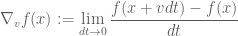 .
.
[Strictly speaking, if X is not flat, then x+vdt is only defined up to an ambiguity of o(dt), but let us ignore this minor issue here, as it is not important in the limit.] If f is sufficiently smooth (being continuously differentiable will do), the directional derivative is linear in v, thus for instance  . One can also generalise the range of f to other multi-dimensional domains than
  ; the directional derivative then lives in a tangent space of that domain.
In all of the above examples, though, we were differentiating functions  , thus each element in the base (or domain) gets mapped to an element in the same range Y. However, in many geometrical situations we would like to differentiate sections
  instead of functions, thus f now maps each point in the base to an element
  of some fibre in a fibre bundle . For instance, one might want to know how the wind direction changes as one moves x in some direction v; thus computing a directional derivative
  of w at x in direction v. One can try to mimic the previous definitions in order to define this directional derivative. For instance, one can move x along v by some infinitesimal amount dt, creating a nearby point
  , and then evaluate w at this point to obtain
  . But here we hit a snag: we cannot directly compare with
  , because the former lives in the fibre
  while the latter lives in the fibre .
With a gauge, of course, we can identify all the fibres (and in particular, and ) with a common object G, in which case there is no difficulty comparing with . But this would lead to a notion of derivative which is not gauge-invariant, known as the non-covariant or ordinary derivative in physics.
But there is another way to take a derivative, which does not require the full strength of a gauge (which identifies all fibres simultaneously together). Indeed, in order to compute a derivative , one only needs to identify (or connect) two infinitesimally close fibres together: and . In practice, these two fibres are already “within O(dt) of each other” in some sense, but suppose in fact that we have some means  of identifying these two fibres together. Then, we can pull back from to through
  to define the covariant derivative:
 .
.
In order to retain the basic property that  is linear in v, and to allow one to extend the infinitesimal identifications
 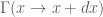 to non-infinitesimal identifications, we impose the property that the to be approximately transitive in that
 (1)
(1)
for all x, dx, dx’, where the  symbol indicates that the error between the two sides is o(|dx| + |dx’|). [The precise nature of this error is actually rather important, being essentially the curvature of the connection
  at x in the directions
  , but let us ignore this for now.] To oversimplify a little bit, any collection of infinitesimal maps obeying this property (and some technical regularity properties) is a connection.
[There are many other important ways to view connections, for instance the Christoffel symbol perspective that we will discuss a bit later. Another approach is to focus on the differentiation operation  rather than the identifications or
  , and in particular on the algebraic properties of this operation, such as linearity in v or derivation-type properties (in particular, obeying various variants of the Leibnitz rule). This approach is particularly important in algebraic geometry, in which the notion of an infinitesimal or of a path may not always be obviously available, but we will not discuss it here.]
The way we have defined it, a connection is a means of identifying two infinitesimally close fibres  of a fibre bundle . But, thanks to (1), we can also identify two distant fibres
  , provided that we have a path
 ![\gamma: [a,b] \to X](https://s0.wp.com/latex.php?latex=%5Cgamma%3A+%5Ba%2Cb%5D+%5Cto+X&bg=ffffff&fg=545454&s=0&c=20201002) from
from  to
to  , by concatenating the infinitesimal identifications by a non-commutative variant of a Riemann sum:
 (2)
(2)
where  ranges over partitions. This gives us a parallel transport map
  identifying with
  , which in view of its Riemann sum definition, can be viewed as the “integral” of the connection along the curve
  . This map does not depend on how one parametrises the path , but it can depend on the choice of path used to travel from x to y.
We illustrate these concepts using several examples, including the three examples introduced earlier.
Example 1 continued. (Circle bundle of the sphere) The geometry of the sphere X in Example 1 provides a natural connection on the circle bundle SX, the Levi-Civita connection , that lets one transport directions around the sphere in as “parallel” a manner as possible; the precise definition is a little technical (see e.g. my lecture notes for a brief description). Suppose for instance one starts at some location x on the equator of the earth, and moves to the antipodal point y by a great semi-circle going through the north pole. The parallel transport  along this path will map the north direction at x to the south direction at y. On the other hand, if we went from x to y by a great semi-circle
  going along the equator, then the north direction at x would be transported to the north direction at y. Given a section u of this circle bundle, the quantity
  can be interpreted as the rate at which u rotates as one travels from x with velocity v.
Example 2 continued. (Circle extensions) In Example 2, we change the notion of “infinitesimally close” by declaring x and Tx to be infinitesimally close for any x in the base space X (and more generally, x and  are non-infinitesimally close for any positive integer n, being connected by the path
  , and similarly for negative n). A cocycle can then be viewed as defining a connection on the skew product , by setting
  (and also
  and
and  to ensure compatibility with (1); to avoid notational ambiguities let us assume for sake of discussion that
  are always distinct from each other). The non-infinitesimal connections
  are then given by the formula
  for positive n (with a similar formula for negative n). Note that these iterated cocycles
  also describe the iterations of the shift
  , indeed
  .
.
Example 3 continued. (Oriented graphs) In Example 3, we declare two edges e, e’ in X to be “infinitesimally close” if they are adjacent. Then there is a natural notion of parallel transport on the bundle ; given two adjacent edges  ,
,  , we let
  be the isomorphism from
  to
to  that maps
  to
to  and
and  to
to  . Any path
  of edges then gives rise to a connection identifying
  with
with  . For instance, the triangular path
  induces the identity map on
  , whereas the U-turn path
  induces the anti-identity map on .
Given an orientation  of the graph G, one can “differentiate”
  at an edge
  in the direction
  to obtain a number
  , defined as +1 if the parallel transport from and
  preserves the orientations given by , and -1 otherwise. This number of course depends on the choice of orientation. But certain combinations of these numbers are independent of such a choice; for instance, given any closed path
  of edges in X, the “integral”
  is independent of the choice of orientation (indeed, it is equal to +1 if is the identity, and -1 if is the anti-identity.
Example 4. (Monodromy) One can interpret the monodromy maps of a covering space in the language of connections. Suppose for instance that we have a covering space of a topological space X whose fibres are discrete; thus is a discrete fibre bundle over X. The discreteness induces a natural connection on this space, which is given by the lifting map; in particular, if one integrates this connection on a closed loop based at some point x, one obtains the monodromy map of that loop at x.
Example 5. (Definite integrals) In view of the definition (2), it should not be surprising that the definite integral  of a scalar function can be interpreted as an integral of a connection. Indeed, set
 ![X := [a,b]](https://s0.wp.com/latex.php?latex=X+%3A%3D+%5Ba%2Cb%5D&bg=ffffff&fg=545454&s=0&c=20201002) , and let
, and let  be the trivial line bundle over X. The function f induces a connection
  on this bundle by setting

The integral ![\Gamma_f([a,b])](https://s0.wp.com/latex.php?latex=%5CGamma_f%28%5Ba%2Cb%5D%29&bg=ffffff&fg=545454&s=0&c=20201002) of this connection along
of this connection along ![{}[a,b]](https://s0.wp.com/latex.php?latex=%7B%7D%5Ba%2Cb%5D&bg=ffffff&fg=545454&s=0&c=20201002) is then just the operation of translation by in the real line.
is then just the operation of translation by in the real line.
Example 6. (Line integrals) One can generalise Example 5 to encompass line integrals in several variable calculus. Indeed, if  is an n-dimensional domain, then a vector field
  induces a connection on the trivial line bundle by setting

The integral  of this connection along a curve is then just the operation of translation by the line integral
  in the real line.
Note that a gauge transformation in this context is just a vertical translation  of the bundle
  by some potential function
  , which we will assume to be smooth for sake of discussion. This transformation conjugates the connection to the connection
  . Note that this is a conservative transformation: the integral of a connection along a closed loop is unchanged by gauge transformation.
Example 7. (ODE) A different way to generalise Example 5 can be obtained by using the fundamental theorem of calculus to interpret ![\int_{[a,b]} f(x)\ dx](https://s0.wp.com/latex.php?latex=%5Cint_%7B%5Ba%2Cb%5D%7D+f%28x%29%5C+dx&bg=ffffff&fg=545454&s=0&c=20201002) as the final value
as the final value  of the solution to the initial value problem
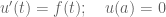
for the ordinary differential equation  . More generally, the solution u(b) to the initial value problem

for some ![u: [a,b] \to {\Bbb R}^n](https://s0.wp.com/latex.php?latex=u%3A+%5Ba%2Cb%5D+%5Cto+%7B%5CBbb+R%7D%5En&bg=ffffff&fg=545454&s=0&c=20201002) taking values in some manifold Y, where
taking values in some manifold Y, where ![F: [a,b] \times {\Bbb R}^n \to {\Bbb R}^n](https://s0.wp.com/latex.php?latex=F%3A+%5Ba%2Cb%5D+%5Ctimes+%7B%5CBbb+R%7D%5En+%5Cto+%7B%5CBbb+R%7D%5En&bg=ffffff&fg=545454&s=0&c=20201002) is a function (let us take it to be Lipschitz, to avoid technical issues), can also be interpreted as the integral of a connection on the trivial vector space bundle
is a function (let us take it to be Lipschitz, to avoid technical issues), can also be interpreted as the integral of a connection on the trivial vector space bundle ![({\Bbb R}^n)_{t \in [a,b]}](https://s0.wp.com/latex.php?latex=%28%7B%5CBbb+R%7D%5En%29_%7Bt+%5Cin+%5Ba%2Cb%5D%7D&bg=ffffff&fg=545454&s=0&c=20201002) , defined by the formula
, defined by the formula

Then ![\Gamma[a,b]](https://s0.wp.com/latex.php?latex=%5CGamma%5Ba%2Cb%5D&bg=ffffff&fg=545454&s=0&c=20201002) will map
will map  to , this is nothing more than the Euler method for solving ODE. Note that the method of integrating factors in solving ODE can be interpreted as an attempt to simplify the connection via a gauge transformation. Indeed, it can be profitable to view the entire theory of connections as a multidimensional “variable-coefficient” generalisation of the theory of ODE.
Once one selects a gauge, one can express a connection in terms of that gauge. In the case of vector bundles (in which every fibre is a d-dimensional vector space for some fixed d), the covariant derivative of a section w of that bundle along some vector v emanating from x can be expressed in any given gauge by the formula

where we use the gauge to express w(x) as a vector  , the indices
  are summed over the fibre dimensions (and summed over the base dimensions) as per the usual conventions, and the
 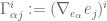 are the Christoffel symbols of this connection relative to this gauge.
One example of this, which models electromagnetism, is a connection on a complex line bundle 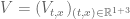 in spacetime
  . Such a bundle assigns a complex line
  (i.e. a one-dimensional complex vector space, and thus isomorphic to
  ) to every point
  in spacetime. The structure group here is U(1) (strictly speaking, this means that we view the fibres as normed one-dimensional complex vector spaces, otherwise the structure group would be
  ). A gauge identifies V with the trivial complex line bundle
  , thus converting sections
  of this bundle into complex-valued functions
  . A connection on V, when described in this gauge, can be given in terms of fields
  for
for  ; the covariant derivative of a section in this gauge is then given by the formula
 .
.
In the theory of electromagnetism,  and
and  are known (up to some normalising constants) as the electric potential and magnetic potential respectively. Sections of V do not show up directly in Maxwell’s equations of electromagnetism, but appear in more complicated variants of these equations, such as the Maxwell-Klein-Gordon equation.
A gauge transformation of V is given by a map  ; it transforms sections by the formula
  , and connections by the formula
  , or equivalently
 . (2)
. (2)
In particular, the electromagnetic potential  is not gauge invariant (which broadly corresponds to the concept of being nonphysical or nonmeasurable in physics), as gauge symmetry allows one to add an arbitrary gradient function to this potential. However, the curvature tensor
![F_{\alpha \beta} := [\nabla_\alpha, \nabla_\beta] = \partial_\alpha A_\beta - \partial_\beta A_\alpha](https://s0.wp.com/latex.php?latex=F_%7B%5Calpha+%5Cbeta%7D+%3A%3D+%5B%5Cnabla_%5Calpha%2C+%5Cnabla_%5Cbeta%5D+%3D+%5Cpartial_%5Calpha+A_%5Cbeta+-+%5Cpartial_%5Cbeta+A_%5Calpha&bg=ffffff&fg=545454&s=0&c=20201002)
of the connection is gauge-invariant, and physically measurable in electromagnetism; the components  for
for  of this field have a physical interpretation as the electric field, and the components
  for
for  have a physical interpretation as the magnetic field. (The curvature tensor
  can be interpreted as describing the parallel transport of infinitesimal rectangles; it measures how far off the connection is from being flat, which means that it can be (locally) “straightened” via some choice of gauge to be the trivial connection. In nonabelian gauge theories, in which the structure group is more complicated than just the abelian group U(1), the curvature tensor is non-scalar, but remains gauge-invariant in a tensor sense (gauge transformations will transform the curvature as they would transform a tensor of the same rank).
Gauge theories can often be expressed succinctly in terms of a connection and its curvatures. For instance, Maxwell’s equations in free space, which describes how electromagnetic radiation propagates in the presence of charges and currents (but no media other than vacuum), can be written (after normalising away some physical constants) as

where  is the 4-current. (Actually, this is only half of Maxwell’s equations, but the other half are a consequence of the interpretation (*) of the electromagnetic field as a curvature of a U(1) connection. Thus this purely geometric interpretation of electromagnetism has some non-trivial physical implications, for instance ruling out the possibility of (classical) magnetic monopoles.) If one generalises from complex line bundles to higher-dimensional vector bundles (with a larger structure group), one can then write down the (classical) Yang-Mills equation

which is the classical model for three of the four fundamental forces in physics: the electromagnetic, weak, and strong nuclear forces (with structure groups U(1), SU(2), and SU(3) respectively). (The classical model for the fourth force, gravitation, is given by a somewhat different geometric equation, namely the Einstein equations  , though this equation is also “gauge-invariant” in some sense.)
The gauge invariance (or gauge freedom) inherent in these equations complicates their analysis. For instance, due to the gauge freedom (2), Maxwell’s equations, when viewed in terms of the electromagnetic potential , are ill-posed: specifying the initial value of this potential at time zero does not uniquely specify the future value of this potential (even if one also specifies any number of additional time derivatives of this potential at time zero), since one can use (2) with a gauge function U that is trivial at time zero but non-trivial at some future time to demonstrate the non-uniqueness. Thus, in order to use standard PDE methods to solve these equations, it is necessary to first fix the gauge to a sufficient extent that it eliminates this sort of ambiguity. If one were in a one-dimensional situation (as opposed to the four-dimensional situation of spacetime), with a trivial topology (i.e. the domain is a line rather than a circle), then it is possible to gauge transform the connection to be completely trivial, for reasons generalising both the fundamental theorem of calculus and the fundamental theorem of ODEs. (Indeed, to trivialise a connection on a line , one can pick an arbitrary origin  and gauge transform each point
  by
by ![\Gamma([t_0,t])](https://s0.wp.com/latex.php?latex=%5CGamma%28%5Bt_0%2Ct%5D%29&bg=ffffff&fg=545454&s=0&c=20201002) .) However, in higher dimensions, one cannot hope to completely trivialise a connection by gauge transforms (mainly because of the possibility of a non-zero curvature form); in general, one cannot hope to do much better than setting a single component of the connection to equal zero. For instance, for Maxwell’s equations (or the Yang-Mills equations), one can trivialise the connection in the time direction, leading to the temporal gauge condition
.) However, in higher dimensions, one cannot hope to completely trivialise a connection by gauge transforms (mainly because of the possibility of a non-zero curvature form); in general, one cannot hope to do much better than setting a single component of the connection to equal zero. For instance, for Maxwell’s equations (or the Yang-Mills equations), one can trivialise the connection in the time direction, leading to the temporal gauge condition
 .
.
This gauge is indeed useful for providing an easy proof of local existence for these equations, at least for smooth initial data. But there are many other useful gauges also that one can fix; for instance one has the Lorenz gauge

which has the nice property of being Lorentz-invariant, and transforms the Maxwell or Yang-Mills equations into linear or nonlinear wave equations respectively. Another important gauge is the Coulomb gauge

where i only ranges over spatial indices 1,2,3 rather than over spacetime indices 0,1,2,3. This gauge has an elliptic variational formulation (Coulomb gauges are critical points of the functional  ) and thus are expected to be “smaller” and “smoother” than many other gauges; this intuition can be borne out by standard elliptic theory (or Hodge theory, in the case of Maxwell’s equations). In some cases, the correct selection of a gauge is crucial in order to establish basic properties of the underlying equation, such as local existence. For instance, the simplest proof of local existence of the Einstein equations uses a harmonic gauge, which is analogous to the Lorenz gauge mentioned earlier; the simplest proof of local existence of Ricci flow uses a gauge of de Turck that is also related to harmonic maps (see e.g. my lecture notes); and in my own work on wave maps, a certain “caloric gauge” based on harmonic map heat flow is crucial (see e.g. this post of mine). But in many situations, it is not yet fully understood whether the use of the correct choice of gauge is a mere technical convenience, or is more innate to the equation. It is definitely conceivable, for instance, that a given gauge field equation is well-posed with one choice of gauge but ill-posed with another. It would also be desirable to have a more gauge-invariant theory of PDEs that did not rely so heavily on gauge theory at all, but this seems to be rather difficult; many of our most powerful tools in PDE (for instance, the Fourier transform) are highly non-gauge-invariant, which makes it very inconvenient to try to analyse these equations in a purely gauge-invariant setting.


60 comments
Comments feed for this article
29 August, 2019 at 2:19 pm
Ray 4.0 : reality of the Virtual – Whereof one cannot speak
[…] a connection so you know how the sections on the manifold on TM evolve in time. Please check out Terry Tao’s post, where he talks about the duality of differential geometry and number theory which splits the […]
13 August, 2021 at 12:11 pm
Anonymous
The usual interpretation of Maxwell’s equations is to assume the 4-current as a (given!) “source” and solve the equations for the 4-potential.
Another possible interpretation is to assume the 4-potential as (given!) “input” which (by Maxwell’s equations) uniquely define(!) the 4-current (as “output”) – thereby interpreting Maxwell’s equations as a mere definition(!) of the 4-current from the 4-potential (without any constraints on the 4-potential).
25 April, 2023 at 7:45 am
Puzzled
Can you explain in more detail why Z/2Z is the structure group for angles?
26 April, 2023 at 11:56 am
Still Puzzled
To elaborate on my question, I get that there is an orientation choice, but don’t we have freedom also choose what angle is equivalent to 0 for instance 360 degrees instead of 2pi radians? Am I missing a constraint here that prevents that?
7 March, 2024 at 12:09 pm
Log-Concavity and Conformal Gauges – Gabe Khan's blog
[…] use gauges in ingenious ways to prove results in geometry and mathematical physics. There is a good blog post by Terry Tao on the topic and another on Uhlenbeck’s work when she won the Abel […]
7 May, 2024 at 11:31 am
Vahid
Dear Prof. Tao
Thank you for this great lecture.
Can you also make a comment on difference between gauge transformations (symmetries) of a system versus global symmetries. We know that the gauge symmetries have trivial (0 or boundary charges) Noether charges while the global symmetrie have non-trivial charges (like energy, …).
It seems that even those boundary charges are also important in gauge theories. For example in general relativity the only acceptable notion of energy is a Noether boundary charge associated to a boundary gauge transformation.
Now, I am confused when you say ”It would also be desirable to have a more gauge-invariant theory of PDEs that did not rely so heavily on gauge theory at all”.
How can we get the same gauge effects (like memory effect) if we do not have them in the first place?