In the first lecture, we introduce flows  on Riemannian manifolds
  , which are recipes for describing smooth deformations of such manifolds over time, and derive the basic first variation formulae for how various structures on such manifolds (e.g. curvature, length, volume) change by such flows. (One can view these formulae as describing the relationship between two “infinitesimally close” Riemannian manifolds.) We then specialise to the case of Ricci flow (together with some close relatives of this flow, such as renormalised Ricci flow, or Ricci flow composed with a diffeomorphism flow). We also discuss the “de Turck trick” that modifies the Ricci flow into a nonlinear parabolic equation, for the purposes of establishing local existence and uniqueness of that flow.
— Flows on Riemannian manifolds —
For the purposes of this course, we are not interested in just a single Riemannian manifold  , but rather a one-parameter family of such manifolds , parameterised by a “time” parameter t. The manifold
  at time t is going to determine the manifold
  at an infinitesimal time t + dt into the future, according to some prescribed evolution equation (e.g. Ricci flow). In order to do this rigorously, we will need to “differentiate” a manifold flow with respect to time.
There are at least two ways to do this. The simplest is to restrict to the case in which the underlying manifold  is fixed (as a smooth manifold), so that only the metric
  varies in time. As g takes values as sections in a vector bundle, there is then no difficulty in defining time derivatives
  in the usual manner:
 . (1)
. (1)
We can of course similarly define the time derivative of any other tensor field by the same formula.
The one drawback of the above simple approach is that it forces the topology of the underlying manifold M to stay constant. A more general approach is to view each d-dimensional manifold M(t) as a slice of a d+1-dimensional “spacetime” manifold  (possibly with boundary or singularities). This spacetime is (usually) equipped with a time coordinate
  , as well as a time vector field
  which obeys the transversality condition
  . The level sets of the time coordinate t then determine the sets M(t), which (assuming non-degeneracy of t) are smooth d-dimensional manifolds which collectively have a tangent bundle
  which is a d-dimensional subbundle of the d+1-dimensional tangent bundle
  of . The metrics g(t) can then be viewed collectively as a section
  of
of  . The analogue of the time derivative
  is then the Lie derivative
  . One can then define other Riemannian structures (e.g. Levi-Civita connections, curvatures, etc.) and differentiate those in a similar manner.
The former approach is of course a special case of the latter, in which  for some time interval
  with the obvious time coordinate and time vector field. The advantage of the latter approach is that it can be extended (with some technicalities) into situations in which the topology changes (though this may cause the time coordinate to become degenerate at some point, thus forcing the time vector field to develop a singularity). This leads to concepts such as generalised Ricci flow, which we will not discuss here, though it is an important part of the definition of Ricci flow with surgery (see Chapters 3.8 and 14 of Morgan-Tian’s book for details). Instead, we focus exclusively for now on the former viewpoint, in which does not depend on time.
Suppose we have a smooth flow  of metrics on a fixed background manifold M. The rate of change of the metric
  is given by
  . By the chain rule, this implies that any other expression that depends on this metric, such as the curvatures
  ,
,  ,
,  , should have a rate of change that depends linearly on . We now compute exactly what these rates of change are. In principle, this can be done by writing everything explicitly using local coordinates and applying the chain rule, but we will try to keep things as coordinate-free as possible as it seems to cut down the computation slightly.
To abbreviate notation, we shall omit the explicit time dependence in what follows, e.g. abbreviating g(t) to just g. We shall call a tensor field w time-independent or static if it does not depend on t, or equivalently that  .
.
From differentiating the identity
 (2)
(2)
we obtain the variation formula
 (3)
(3)
(here is a place where the raising and lowering conventions can be confusing if applied blindly!).
Next, we compute how covariant differentiation deforms with respect to time. For a scalar function f, the derivative  does not involve the metric, and so the rate of change formula is simple:
 . (4)
. (4)
In particular, if f is static, then so is  .
.
Now we take a static vector field  . From (4) and the product rule we see that the expression
  is linear over
  (interpreted as the space of static scalar fields). Thus we must have
 (5)
(5)
for some rank (1,2) tensor  . From the Leibnitz rule and (4) we can obtain similar formulae for other tensors, e.g.
 (5′)
(5′)
for any static one-form  .
.
What is  ? Well, we can work it out from the properties of the Levi-Civita connection. Differentiating the torsion-free identity
 (6)
(6)
for static scalar fields f using (4), (5′), we conclude the symmetry  . Similarly, differentiating the respect-of-metric identity
  we conclude that
 . (7)
. (7)
These two facts allow us to solve for :
 (8)
(8)
(compare with the usual formula for the Christoffel symbols in local coordinates).
Now we turn to curvature tensors. We have the identity
 (9)
(9)
for any static vector field X. Taking the time derivative of this using (5), (5′), etc. we obtain


 (10)
(10)
which eventually simplifies to
 . (11)
(one can view this as a linearisation of the usual formula for the Riemann curvature tensor in terms of Christoffel symbols). Combining (8) and (11), and using the fact that the Levi-Civita connection respects the metric, we thus have

 (12)
(12)
Exercise 1. Show that (12) is consistent with the antisymmetry properties of the Riemann tensor, and with the Bianchi identities, as presented in the previous lecture. 
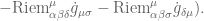
Taking traces, we obtain a variation formula for the Ricci tensor
 (13)
(13)
where  is the trace, and the Lichnerowicz Laplacian (or Hodge-de Rham Laplacian)
  on symmetric rank (0,2) tensors
  is defined by the formula
 (14)
(14)
and  is the usual connection Laplacian. Taking traces once again, one obtains a variation formula for the scalar curvature:
 . (15)
Exercise 2. Verify the derivation of (13) and (15). [Aside: – I wonder if there are more direct derivations of (13) and (15) that do not require one to go through so many computations. One can use (22) and (26) below as consistency checks for these formulae, but this does not quite seem sufficient.]
We will also need to understand how deformation of the metric affects two other quantities, length and volume. The length  of a curve
 ![\gamma: [a,b] \to M](https://s0.wp.com/latex.php?latex=%5Cgamma%3A+%5Ba%2Cb%5D+%5Cto+M&bg=ffffff&fg=545454&s=0&c=20201002) in a Riemannian manifold is given by the formula
in a Riemannian manifold is given by the formula
 . (16)
where  is the measure on the curve
  induced by the metric.
Exercise 3. If varies smoothly in time (but with static endpoints  , show that
 (17)
(17)
where at every point  of the curve,
  is the unit tangent, and
  is the variation field. (Strictly speaking, one needs to work on the pullback tensor bundles on
 ![{}[a,b]](https://s0.wp.com/latex.php?latex=%7B%7D%5Ba%2Cb%5D&bg=ffffff&fg=545454&s=0&c=20201002) rather than M in order to make the formulae in (17) well defined.)
rather than M in order to make the formulae in (17) well defined.)
The distance between two points x, y on a manifold is defined as  , where ranges over all curves from x to y. For smooth connected complete manifolds, it is not hard to show (e.g. by using a reduction to the unit speed case, followed by a minimising sequence argument and the Arzelà-Ascoli theorem, combined with some local theory of short geodesics to ensure
  regularity of the limiting curve) that this infimum is actually attained for some minimising geodesic , which is then a critical point for . (However, this infimum need not be unique if x, y are far apart.) From (17) we conclude that such geodesics must obey the equation
  (thus the unit tangent vector parallel transports itself). We also conclude that
 (18)
(18)
where the infimum is over all the minimising geodesics from x to y. Thus, a positive  (in the sense of quadratic forms) will increase distances between two marked points, while a negative will decrease it.
Next, we look at the evolution of the volume measure  . This measure is defined using any frame
  and dual frame
  as
as
 (18′)
(18′)
where  is the determinant of the matrix with components
  (one can check that this measure is defined independently of the choice of frame). Intuitively, this measure is the unique measure such that an infinitesimal cube whose sides are orthogonal vectors of infinitesimal length
  , will have volume
  . It is not hard to show (using coordinates, and the variation formula
 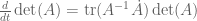 for the determinant) that one has
 . (19)
Thus, a positive trace for implies volume expansion, and a negative trace implies volume contraction. This is broadly consistent with how length is affected by metric distortion, as discussed previously.
— Dilations —
Now we specialise to some specific flows  of a Riemannian metric on a fixed background manifold M. The simplest such flow (besides the trivial flow
  , of course) is that of a dilation
 (20)
(20)
where  is a positive scalar with
  . The flow here is given by
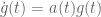 (21)
(21)
where 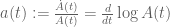 is the logarithmic derivative of A (or equivalently,
  ). In this case our variation formulas become very simple:


 (22)
(22)


 ;
;
note that these formulae are consistent with (20) and the scaling heuristics at the end of the previous lecture. In particular, a positive value of  means that length and volume are increasing, and a negative value means that length and volume are decreasing.
— Diffeomorphisms —
Another basic flow comes from smoothly varying one-parameter families of diffeomorphisms  with
with  equal to the identity. This induces a flow
 (23).
(23).
Infinitesimally, this flow is given by the Lie derivative
 (24)
(24)
where  is the vector field representing the infinitesimal diffeomorphism at time t. (One can use Picard’s existence theorem to recover
  from X, though one has to solve an ODE for this and so the formula is not fully explicit.) The quantity
  is known as the deformation tensor of X, and it is a short exercise to verify the identity
 . (25)
(Informally, this tensor measures the obstruction to K being a Killing vector field.)
It is clear from diffeomorphism invariance that all tensors deform via the Lie derivative:

 (26)
(26)
 .
.
[The formula for does not have such a nice representation, since  is not a tensor.]
Exercise 4. Establish the first variation formula  , where the infimum ranges over all minimal geodesics from x to y (which in particular determine the unit tangent vector S at x and at y).
Remark 1. As observed by Kazdan, one can compare the identities (26) with the variation formulae (11), (13), (15) to provide an alternate derivation of the Bianchi identities.
Applying (19), (25) we see that variation of the volume measure  is given by
 (27)
(27)
where  is the divergence of X. On the other hand, for compact manifolds M at least, diffeomorphisms preserve the total volume
  . We thus conclude Stokes’ theorem
 (28)
(28)
on compact manifolds for arbitrary smooth vector fields X. It is not difficult to extend this to non-compact manifolds in the case when X is compactly supported. From (28) and the product rule we also obtain the integration by parts formula
 . (29)
As one particular special case of (29), we observe that the Laplacian on is formally self-adjoint.
— Ricci flow —
Finally, we come to the main focus of this entire course, namely Ricci flow. A one-parameter family of metrics g(t) on a smooth manifold M for all time t in an interval I is said to obey Ricci flow if we have
 . (30)
Note that this equation makes tensorial sense since g and Ric are both symmetric rank 2 tensors. The factor of 2 here is just a notational convenience and is not terribly important, but the minus sign – is crucial (at least, if one wants to solve Ricci flow forwards in time). Note that Ricci flow, like all other parabolic flows (of which the heat equation is the model example), is not time-reversible – solvability forwards in time does not imply solvability backwards in time!
In the preceding examples of dilation flow and diffeomorphism flow, it was easy to get from the infinitesimal evolution to the global evolution, either by using an integrating factor or by solving some ODEs. The situation for Ricci flow turns out to be significantly less trivial (and indeed, resolving the global existence problem properly is a large part of the proof of the Poincaré conjecture). Nevertheless, we do have the following relatively easy result:
Theorem 1 (local existence). If M is compact and  is a smooth Riemannian metric on M, then there exists a time
  , and a unique Ricci flow
  with initial metric g(0) on the time interval
  .
.
This theorem was first proven by Hamilton using the Nash-Moser iteration method, and then a simplified proof given by de Turck. We will not prove Theorem 1 here, but we will shortly indicate the main trick of de Turck used to reduce the problem to a standard local existence problem for nonlinear parabolic PDE.
Solutions have various names depending on their interval I of existence (or lifespan):
- A solution is ancient if I has
 as a left endpoint.
- A solution is immortal if I has
 as a right-endpoint.
- A solution is global if it is both ancient and immortal, thus
 .
.
The ancient solutions will play a particularly important role in our analysis later in this course, when we rescale (or blow up) the time variable (and the metric) as we approach a singularity of the Ricci flow, and then look at the asymptotic limiting profile of these rescaled solutions.
It is a routine matter to compute the variations of various tensors under the Ricci flow:

 (31)
(31)


where  is a moderately complicated combination of the tensors
  , Riem, and Riem that I will not write down explicitly here. In particular, we see that all of the curvature tensors obey some sort of tensor nonlinear heat equation. Parabolic theory then suggests that these tensors will behave for short times much like solutions to the linear heat equation (for instance, they should become smoother over time, and they should obey various maximum principles). We will see various manifestations of this principle later in this course.
We also have variation formulae for length and volume:
 (32)
(32)
 . (33)
Thus Ricci flow tends to enlarge length and volume in regions of negative curvature, and reduce length and volume in regions of positive curvature.
— Modifying Ricci flow —
Ricci flow (30) combines well with the dilation flows (21) and diffeomorphism flows (24), thanks to the dilation symmetry and diffeomorphism invariance of Ricci flow. (It can even be combined with these two flows simultaneously, although we will not need such a unified flow here.)
For instance, if g(t) solves Ricci flow and we set  for some reparameterised time
  and some scalar
  , then the Ricci curvature here is
  . We then see from the chain rule that
  obeys the equation
 (34)
(34)
where is the logarithmic derivative of A. If we normalise the time reparameterisation by requiring  , we thus see that obeys normalised Ricci flow
 (35)
(35)
which can be viewed as a combination of (30) and (21). Conversely, it is not difficult to reverse these steps and transform a solution to (35) for some a into a solution of Ricci flow by reparameterising time and renormalising the metric by a scalar. Normalised Ricci flow is useful for studying singularities, as it can “blow up” the interesting portion of the dynamics to keep it at unit scale, instead of cascading to finer and finer scales as is usual when approaching a singularity. The parameter a is at one’s disposal to set; for instance, one could choose a to normalise the volume of M to be constant, or perhaps to normalise the maximum scalar curvature  to be constant. (Of course, only one quantity at a time can be normalised to be constant, since one only has one free parameter to set.)
Setting a=0, we observe in particular that the solution space to Ricci flow enjoys the scaling symmetry
 (36)
(36)
for any  . Thus, if we enlarge a manifold M by
  (or equivalently, if we fix M but make the metric g
  times as large), then Ricci flow will become slower by a factor of , and conversely if we shrink a manifold by then Ricci flow speeds up by . Thus, as a first approximation, big manifolds tend to evolve slowly under Ricci flow, and small ones tend to evolve quickly.
Similarly, Ricci flow combines well with diffeomorphisms. If g(t) solves Ricci flow and is a smoothly varying family of diffeomorphisms, then we can define a modified Ricci flow  (cf. (23)). As Ricci curvature is intrinsic, this new metric has curvature
  . It is then not hard to see that evolves by the flow
 (36′)
(36′)
where  are the vector fields that direct the flow as before. Note that (36′) is a combination of (30) and (24). Conversely, given a solution to a modified Ricci flow (36′) for some smoothly time-varying vector field X, one can convert it back to a Ricci flow by solving for the diffeomorphisms and then using them as a change of variables.
The modified flows (36′) (with various choices of vector field X) arise in a number of contexts. For instance, they are useful for studying gradient Ricci solitons, which will be an important special solution to Ricci flow that we will encounter later. Also, modified Ricci flow is an excellent tool for assisting the proof of local existence (Theorem 1), because it can be used (via the “de Turck trick”) to “gauge away” some nasty non-parabolic components in Ricci flow, leaving behind a nicely parabolic non-linear PDE known as Ricci-de Turck flow which is straightforward to solve.
To explain this, let us first write the Ricci flow equation (30) “in coordinates” in order to attempt to solve it as a nonlinear PDE. (The current state of the art of PDE existence theory does not cope all that well with the coordinate-independent frameworks which are embraced by differential geometers; in order to demonstrate existence of just about any equation, one usually has to break the covariance of the situation, and pick some coordinate system to work with. On the other hand, for particularly geometric equations, such as Ricci flow, there are often some special coordinate systems that one can pick that will simplify the PDE analysis enormously.)
The traditional way to express Ricci flow in coordinates is, of course, to use local coordinate charts, but let us present a slightly different way to do this, relying on an arbitrarily chosen background metric  on M which does not depend on time. (For instance, one could pick
  to be the initial metric, although we do not need to do so.) This gives us a background connection
  , background curvature tensors
  , and so forth. One can then express the evolving metric in terms of the background by a variety of formulae. For instance, the evolving connection
  can be expressed in terms of the background connection by the formula
 (37)
(37)
where the Christoffel symbol  is given by
 . (38)
Exercise 5. Verify (37) and (38). Then use these formulae to give an alternate derivation of (5) and (8).
From (37) and the definition of Riemann curvature one concludes that

 . (39)
Contracting this, we conclude
 . (40)
Inserting (38) and only keeping careful track of the top order terms, we can eventually rewrite (40) as
 (41)
(41)
where X is the vector field
 . (42)
Exercise 6. Show that the expression (41) for the Ricci curvature can be used to imply (13). Conversely, use (13) to recover (41) without performing an excessive amount of explicit computation. (Hint: first show that the Ricci tensor can be crudely expressed as  .)
.)
Thus, if we happen to have a solution g to modified Ricci flow (36′) with the vector field X given by (42), then the equation (36′) simplifies to the Ricci-de Turck flow
 . (43)
Conversely, it is not too difficult to reverse these steps and convert a solution to Ricci-de Turck flow to a solution to Ricci flow.
The equation (43) is a quasilinear parabolic evolution equation on g (which we think of now as evolving on a fixed background Riemannian manifold  , and one can establish local existence for (43) by a variety of methods. From this and the preceding remarks one can eventually establish Theorem 1, although we will not do so in detail here.
Remark 2. (This remark is intended primarily for experts in nonlinear PDE.) One particular way to establish existence for Ricci-de Turck flow (and probably not the most efficient) is sketched as follows. If one writes  , then one can recast (43) as a heat equation against the fixed background metric that takes the form
 (44)
(44)
for some smooth function F depending on the background (assuming that h is small in  norm so that one can compute the inverse
  smoothly). The essentially semilinear equation (44) can be solved (for initial data small and smooth, and on small time intervals) on a compact manifold M by, say, the Picard iteration method, based on estimates such as the energy inequality
 (45)
(45)
for some suitably large integer k ( will do), and with implied constants depending on the background metric, whenever u is a tensor that solves the heat equation
  . This energy estimate can be easily established by integration by parts. To expand in a little more detail: the Picard iteration method proceeds by constructing iterative approximations
  to a solution h of (44) by solving a sequence of inhomogeneous heat equations
 (44′)
(44′)
starting from  (say). The main task is to show that the sequence
  converges rapidly to zero in a suitable function space, such as
  . This can be done by applying (45) with
  or
or  , and also using some product estimates in Sobolev spaces that are ultimately based on the Sobolev embedding theorem.
There is the still the issue of how to establish existence for the linear heat equation on tensors, but this can be done by functional calculus (once one establishes that  is a genuinely self-adjoint operator), or by making a reasonably accurate parametrix for the heat kernel. One (minor) advantage of this Picard iteration based approach is that it allows one to establish uniqueness and continuous dependence on initial data as well as just existence, and to show that the nonlinear solution obeys similar estimates (locally in time) to that of the linear heat equation. But uniqueness and continuity will not be necessary for the arguments in this course, and the estimates we need can always be established a posteriori by energy inequalities anyway.
Remark 3. The diffeomorphisms needed to convert solutions to Ricci-de Turck flow (43) back to solutions of Ricci flow (30) themselves obey a pleasant evolution equation; in fact, they evolve by harmonic map heat flow from the fixed domain  to the target . See Chapter 3.4 of Chow and Knopf’s book “Ricci Flow: an introduction” for further discussion. More generally, it seems that harmonic maps (and harmonic map heat flow, and harmonic coordinates) often provide natural coordinate systems that make various geometric PDE analytically tractable. On the other hand, for geometric arguments it seems better to work with the original Ricci flow; the de Turck diffeomorphisms seem to obscure many of the delicate monotonicity properties that are essential to the deeper understanding of Ricci flow, and are also not completely covariant as they rely on an arbitrary choice of background metric .
[Update, Apr 3: Minor corrections.]


66 comments
Comments feed for this article
12 January, 2023 at 3:48 pm
Existence of minimizing geodesic – Mathematics – Forum
[…] have read in a post in Terence Tao's blog that in every connected smooth manifold, any two points can be joined by $C^1$-piecewise minimising […]