I was asked recently (in relation to my recent work with Van Vu on the spectral theory of random matrices) to explain some standard heuristics regarding how the eigenvalues  of an
of an  matrix A behave under small perturbations. These heuristics can be summarised as follows:
- For normal matrices (and in particular, unitary or self-adjoint matrices), eigenvalues are very stable under small perturbations. For more general matrices, eigenvalues can become unstable if there is pseudospectrum present.
- For self-adjoint (Hermitian) matrices, eigenvalues that are too close together tend to repel quickly from each other under such perturbations. For more general matrices, eigenvalues can either be repelled or be attracted to each other, depending on the type of perturbation.
In this post I would like to briefly explain why these heuristics are plausible.
— Pseudospectrum —
As any student of linear algebra knows, the spectrum  of a matrix A consists of all the complex numbers
  such that
  fails to be invertible, thus there exists a non-zero vector v such that
  is zero. This is a finite set, consisting of at most n points. But there is also an important set containing the spectrum (and which, at times, can be much larger than that spectrum), which is the pseudospectrum of the matrix A. Unlike the spectrum, which is canonically defined, there is more than one definition of the pseudospectrum; also, this concept depends on an additional parameter, a small number
  . We will define the pseudospectrum (or more precisely, the
  -pseudospectrum)
  to be the set of all the complex numbers such that has least singular value at most , or equivalently that there exists a unit vector v such that
  . (Another equivalent definition is that the -pseudospectrum consists of the spectrum, together with those complex numbers for which the resolvent
  has operator norm at least
  .)
.)
The significance of the pseudospectrum is that it describes where the spectrum can go to under small perturbations. Indeed, if lies in the pseudospectrum , so that there exists a unit vector v whose image  has magnitude at most , then we see that

and so lies in the spectrum  of the perturbation
  of A. Note that the operator norm of
  is at most .
Conversely, if does not lie in the pseudospectrum , and  is a small perturbation of A (with E having operator norm at most ), then for any unit vector v, one has

by the triangle inequality, and so cannot lie in the spectrum of .
Thus, if the pseudospectrum is tightly clustered around the spectrum, the spectrum is stable under small perturbations; but if the pseudospectrum is widely dispersed, then the spectrum becomes unstable.
No matter what A is, the pseudospectrum always contains the -neighbourhood of the spectrum . Indeed, if v is a unit eigenvector with eigenvalue  , then
  , which implies that
  for any
  in the -neighbourhood of , and the claim follows.
Conversely, when A is normal, consists only of the -neighbourhood of . This is easiest to see by using the spectral theorem to diagonalise A and then computing everything explicitly. In particular, we conclude that if we perturb a normal matrix by a (possibly non-normal) perturbation of operator norm at most , then the spectrum moves by at most .
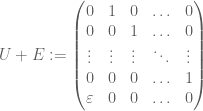
In the non-normal case, things can be quite different. A good example is provided by the shift matrix
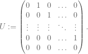
This matrix is nilpotent:  . As such, the only eigenvalue is zero. But observe that for any complex number ,
 .
.
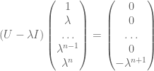
From this and a little computation, we see that if  , then will lie in the
  -pseudospectrum of U. For fixed , we thus see that
  fills up the unit disk in the high dimensional limit
  . (The pseudospectrum will not venture far beyond the unit disk, as the operator norm of U is 1.) And indeed, it is easy to perturb U so that its spectrum moves far away from the origin. For instance, observe that the perturbation
of U has a characteristic polynomial of  (or note that
  , which is basically the same fact thanks to the Cayley-Hamilton theorem) and so has eigenvalues equal to the
  roots of ; for fixed and n tending to infinity, this spectrum becomes asymptotically uniformly distributed on the unit circle, rather than at the origin.
[Update, Nov 8: Much more on the theory of pseudospectra can be found at this web site; thanks to Nick Trefethen for the link.]
— Spectral dynamics —
The pseudospectrum tells us, roughly speaking, how far the spectrum of a matrix A can move with respect to a small perturbation, but does not tell us the direction in which the spectrum moves. For this, it is convenient to use the language of calculus: we suppose that A=A(t) varies smoothly with respect to some time parameter t, and would like to “differentiate” the spectrum with respect to t.
Since it is a little unclear what it means to differentiate a set, let us work instead with the eigenvalues  of
of  . Note that generically (e.g. for almost all A), the eigenvalues will be distinct. (Proof: the eigenvalues are distinct when the characteristic polynomial has no repeated roots, or equivalently when the resultant of the characteristic polynomial with its derivative is non-zero. This is clearly a Zariski-open condition; since the condition is obeyed at least once, it is thus Zariski-dense.) So it is not unreasonable to assume that for all t in some open interval, the
  are distinct; an application of the implicit function theorem then allows one to make the smooth in t. Similarly, we can make the eigenvectors
  vary smoothly in t. (There is some freedom to multiply each eigenvector by a scalar, but this freedom will cancel itself out in the end, as we are ultimately interested only in the eigenvalues rather than the eigenvectors.)
The eigenvectors  form a basis of
  . Let
. Let  be the dual basis, thus
  for all
  , and so we have the reproducing formula
 (1)
(1)
for all vectors u. Combining this with the eigenvector equations
 (2)
(2)
we obtain the adjoint eigenvector equations
 . (3)
. (3)
Next, we differentiate (2) using the product rule to obtain
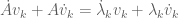 . (4)
. (4)
Taking the inner product of this with the dual vector  , and using (3) to cancel some terms, we obtain the first variation formula for eigenvalues:
 . (5)
. (5)
Note that if A is normal, then we can take the eigenbasis  to be orthonormal, in which case the dual basis is identical to . In particular we see that
  ; the infinitesimal change of each eigenvalue does not exceed the infinitesimal size of the perturbation. This is consistent with the stability of the spectrum for normal operators mentioned in the previous section.
[Side remark: if A evolves by the Lax pair equation ![\dot A = [A,P]](https://s0.wp.com/latex.php?latex=%5Cdot+A+%3D+%5BA%2CP%5D&bg=ffffff&fg=545454&s=0&c=20201002) for some matrix
for some matrix  , then
  , and so from (5) we see that the spectrum of A is invariant in time. This fact underpins the inverse scattering method for solving integrable systems.]
Now we look at how the eigenvectors vary. Taking the inner product instead with a dual vector  for
for  , we obtain
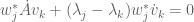 ;
;
applying (1) we conclude a first variation formula for the eigenvectors , namely that
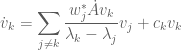 (6)
(6)
for some scalar  (the presence of this term reflects the freedom to multiply by a scalar). Similar considerations for the adjoint give
 (6′)
(6′)
(here we use the derivative of the identity  to get the correct multiple of
  on the right.)
We can use (5), (6), (6′) to obtain a second variation formula for the eigenvalues. Indeed, by differentiating (5) we obtain
 ;
;
applying (6), (6′) we conclude the second variation formula
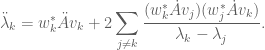 (7)
(7)
Now suppose that A is self-adjoint, so as before we can take  to be orthonormal. The above formula then becomes

One can view the terms on the right-hand side here as various “forces” acting on the eigenvalue  ; the acceleration of the original matrix A provides one such force, while all the other eigenvalues
  provide a repulsive force (and note, as with Newton’s third law, that the force that exerts on is equal and opposite to the force that exerts on ; this is consistent with the trace formula
  ). The closer two eigenvalues are to each other, the stronger the repulsive force becomes.
When the matrix A is not self-adjoint, then the interaction between and can be either repulsive or attractive. Consider for instance the matrices

The eigenvalues of this matrix are  for
for  – so we see that they are attracted to each other as t evolves, until the matrix becomes degenerate at
  . In contrast, the self-adjoint matrices

have eigenvalues  , which repel each other as t evolves.
The repulsion effect of eigenvalues is also consistent with the smallness of the set of matrices with repeated eigenvalues. Consider for instance the space of Hermitian matrices, which has real dimension  . The subset of Hermitian matrices with distinct eigenvalues can be described by a collection of n orthogonal (complex) one-dimensional eigenspaces (which can be computed to have
  degrees of freedom) plus n real eigenvalues (for an additional n degrees of freedom), thus the set of matrices with distinct eigenvalues has full dimension .
Now consider the space of matrices with one repeated eigenvalue. This can be described by n-2 orthogonal complex one-dimensional eigenspaces, plus a complex two-dimensional orthogonal complement (which has  degrees of freedom) plus n-1 real eigenvalues, thus the set of matrices with repeated eigenvalues only has dimension
  . Thus it is in fact very rare for eigenvalues to actually collide, which helps explain why there must be a repulsion effect in the first place.
An example can help illustrate this phenomenon. Consider the one-parameter family of Hermitian matrices

The eigenvalues of this matrix at time t are of course t and -t, which cross over each other when t changes sign. Now consider instead the Hermitian perturbation

for some small . The eigenvalues are now  and
and  ; they come close to each other as t approaches 0, but then “bounce” off of each other due to the repulsion effect.


52 comments
Comments feed for this article
28 October, 2008 at 10:05 am
Anonymous
Dear Terry,
thanks for the nice post! By the way, let me make a suggestion (if you permit): after reading your post, I thought that you could complement it with a few comments about the stability of the spectrum in the infinite dimensional case, e.g., the results of Feldmann, Trubowitz and Knorrer about perturbations of the form of Laplacian
  on the d-dimensional torus (if you are able to find the time to write it down of course).
Bests,
Matheus
28 October, 2008 at 2:24 pm
Terence Tao
Dear Matheus,
I was not familiar with the work of Feldmann et al., but in any event one can understand the spectral theory of self-adjoint unbounded operators such as by viewing them as the limit of the finite-dimensional self-adjoint truncations
  , where
  is a Fourier projection to all modes of size less than N; the spectral theorem for
  shows that any finite number of eigenvalues and eigenvectors of the latter converge to the former in the limit
  (one can also use the minimax formulae for these eigenvalues and eigenvectors here). So any stability statement concerning a bounded number of finite-dimensional eigenvalues or eigenvectors which is uniform in N can be recovered in this infinite-dimensional limit (in principle, at least).
A version of the first variation formula for eigenvalues of Laplacians was used recently by Hassell in his proof of the scarring conjecture for generic Bunimovich stadia, see
29 October, 2008 at 8:57 pm
orr
Dear Prof. Tao,
Is it possible that you meant to write, in the definition of the pseudospectrum, that it is the set of all numbers for which the resolvent has operator norm AT LEAST (and not AT MOST) one over epsilon?
29 October, 2008 at 9:33 pm
Terence Tao
Dear orr: thanks for the correction!
30 October, 2008 at 4:13 pm
Top Posts « WordPress.com
[…] When are eigenvalues stable? I was asked recently (in relation to my recent work with Van Vu on the spectral theory of random matrices) to explain […] […]
31 October, 2008 at 8:49 am
Carlos Matheus
Dear Terry,
this approach (ie, either approximation by finite dimensional self-adjoint operators or minimax principle) works well for the issue of stability of a bounded part of the spectrum in general. Also, we can push this argument to make it work for the whole spectrum in the 1d ‘torus’ case (this is particularly important when dealing with the KAM theory of NLS). In fact, the case of the circle is a bit special because the eigenvalues are simple and they have a ‘good spacing’ (ie the distance between two consecutive eigenvalues grows linearly).
Of course, these two facts are not true for higher dimensional tori. However, Feldman, Trubowitz and Knorrer manage to show in dimensions 2 and 3 (for the usual ‘square, flat’ torus and also for a ‘generic’ torus obtained from a typical lattice) that ‘most’ of eigenvalues are stable (in the sense that the set of stable eigenvalues form a subset of density 1 of the set of eigenvalues). Moreover, they constructed examples where the set of unstable eigenvalues is ‘non-trivial’ (although it has zero density). In particular, this is a technical problem if one would like to show KAM results for the NLS in higher dimensions.
By the way, the references for the papers of Feldman et al. are the following:
Stability results: ”The perturbatively stable spectrum of a periodic Schrödinger operator”. Invent. Math. 100 (1990), no. 2, 259–300.
Instability results: ”Perturbatively unstable eigenvalues of a periodic Schrödinger operator”. Comment. Math. Helv. 66 (1991), no. 4, 557–579.
Bests,
Matheus
3 November, 2008 at 11:21 pm
Jonathan Vos Post
Is there a connection between this approach and the new submissions for Tue, 4 Nov 08
arXiv:0811.0007
Title: Large gaps between random eigenvalues
Authors: Benedek Valkó, Bálint Virág
Comments: 18 pages, 1 figure
Subjects: Probability (math.PR)
We show that in the point process limit of the bulk eigenvalues of $\beta$-ensembles of random matrices, the probability of having no eigenvalue in a fixed interval of size $\lambda$ is given by $$ (\kappa_\beta+o(1))\lambda^{\gamma_\beta} \exp(- \frac{\beta}{64}\lambda^2+(\frac{\beta}{4}-\frac18)\lambda) $$ as $\lambda\to\infty$, where $$ \gamma_\beta={1/4}(\frac\beta{2}+\frac{2}{\beta}- 3). $$ This is a slightly corrected version of a prediction by Dyson. Our proof uses the new Brownian carousel representation of the limit process, as well as the Cameron-Martin-Girsanov transformation in stochastic calculus.
7 November, 2008 at 10:36 am
Carnival of Mathematics #43 « The Number Warrior
[…] of Terence Tao, I recommend his recent post on when eigenvalues are stable. If you’re intimidated by some of his other posts (say, his 19-part series on Ricci flow and […]
8 November, 2008 at 8:59 am
E Brian Davies
Terry’s articles about the uses of pseudospectra touches on what is now a substantial research field. The book by Trefethen and Embree: Spectra and Pseudospectra, Princeton University Press, 2005, provides a wide range of theorems and real-world examples of their application. My own book, Linear Operators and Their Spectra, CUP 2007, is written at a more pure-mathematical level and has a chapter devoted to pseudospectra and what are often called nonlinear generalizations. Terry’s example of a small perturbation of a large Jordan matrix has been explored in detail by M Hager and myself — several relevant papers are in the arXiv.
It is generally considered that theorems about pseudospectra have nicer formulations if one defines the epsilon pseudospectrum using a strict inequality rather than a non-strict one.
8 November, 2008 at 10:42 am
E Brian Davies
With reference to the communications between Terry and Matheus above.
One has to be very careful about computing the spectrum of a self-adjoint operator H by looking at the limit of the spectra of as
as  .
.
This can be justified by a minimax argument if one restricts attention to the part of the spectrum below the essential spectrum. It almost always gives a completely wrong answer if the operator H has a gap between two parts of the essential spectrum. The truncations seem to suggest that the gap is not present. This applies in particular to Schrodinger operators with periodic potentials acting in , which generally have a band-gap structure to the spectrum. If
  is an increasing sequence of finite rank projections constructed by standard finite element methods and converging strongly to the identity operator, then the spectra of the truncations fill up the gaps more and more densely as
  .
.
Once again there is a substantial numerical and analytic literature explaining why this method does not work and what one should do to get the right answer.
9 November, 2008 at 12:50 am
E Brian Davies
More dangers of truncation. I should have mentioned the many papers, indeed books, of Albrecht Boettcher and his co-workers on infinite non-self-adjoint bounded Toeplitz matrices. The spectra of the obvious finite truncations do converge as N\to\infty, but the limits are completely different from the spectra of the infinite matrices. This is a large and fascinating subject, but the message is the same – do not trust truncation unless you actually know that it works in your particular context.
17 November, 2008 at 5:26 pm
me
Also, you may want to check out the papers of Burke, Lewis, and Overton. Together (and apart) they have many papers on Matrix stability, pseudospectral subdifferentials, etc. All very interesting and related work.
9 April, 2009 at 3:37 pm
Steven Heilman
Hi-
I think I found a few errors (most likely due to transcription?):
1. Eq. (3) is missing a * on the right hand side
2. after Eq. (6), should read “… freedom to multiply v_{k}…”
Best-
-Steve
[Corrected, thanks – T.]
28 April, 2009 at 5:53 pm
Tusarepides
Hi, there unfortunately seems to be plenty of formulae that do not parse on this page – I have no trouble with other pages on your blog. Any hints on how I could fix this?
3 June, 2009 at 11:19 am
Random matrices: universality of local eigenvalue statistics « What’s new
[…] of the matrix, and the unit eigenvector of the matrix associated to that eigenvalue. (See this earlier blog post for further discussion of this and related formulae). If one assumes that the eigenvectors are […]
16 August, 2009 at 8:43 am
Random matrices: Universality of local eigenvalue statistics up to the edge « What’s new
[…] eigenvalues of “repel” the eigenvalues of (cf. the eigenvalue repulsion discussed in this previous blog post). On the other hand, the term on the right-hand side of (3) can be viewed as an attractive force […]
12 January, 2010 at 9:03 pm
254A, Notes 3a: Eigenvalues and sums of Hermitian matrices « What’s new
[…] (and also proportional to the square of the matrix coefficient of in the eigenbasis). See this earlier blog post for more discussion. Remark 4 In the proof of the four moment theorem of Van Vu and myself, […]
2 February, 2010 at 1:35 pm
254A, Notes 4: The semi-circular law « What’s new
[…] In a similar vein, we may apply the truncation argument (much as was done for the central limit theorem in Notes 2) to reduce the semi-circular law to the bounded case: Exercise 5 Show that in order to prove the semi-circular law (in the almost sure sense), it suffices to do so under the additional hypothesis that the random variables are bounded. Similarly for the convergence in probability or in expectation senses. Remark 2 These facts ultimately rely on the stability of eigenvalues with respect to perturbations. This stability is automatic in the Hermitian case, but for non-symmetric matrices, serious instabilities can occur due to the presence of pseudospectrum. We will discuss this phenomenon more in later lectures (but see also this earlier blog post). […]
10 February, 2010 at 10:56 pm
245A, Notes 5: Free probability « What’s new
[…] (This is ultimately due to the stable nature of eigenvalues in the self-adjoint setting; see this previous blog post for discussion.) For non-self-adjoint operators, free probability needs to be augmented with […]
7 April, 2010 at 11:12 pm
Hoda
Hi,
From the post:
“1.For normal matrices (and in particular, unitary or self-adjoint matrices), eigenvalues are very stable under small perturbations. For more general matrices, eigenvalues can become unstable if there is pseudospectrum present.”
A question: Does this result also apply for the genralized eigenvalue problem? (Ax = λBx)
Thank you for your help,
Hoda
8 April, 2010 at 8:07 am
Terence Tao
Well, if B is invertible (and well-conditioned), one can recast the generalised eigenvalue problem as an eigenvalue problem for . In general, one does not expect this matrix to have any good properties unless A, B happen to lie in the same Lie group (e.g. they are both unitary), or if A and B commute. But in general (e.g. if A, B are generic Hermitian matrices, whose eigenspaces are “skew” with respect to each other) the problem could be highly unstable in the worst-case scenario (though perhaps only moderately unstable in the average-case scenario, thanks to the smoothed analysis phenomenon).
9 April, 2010 at 2:14 am
Anonymous
Thank you for your explanation
Hoda
22 December, 2010 at 9:08 pm
Outliers in the spectrum of iid matrices with bounded rank permutations « What’s new
[…] non-Hermitian matrices were quite unstable with respect to general perturbations (as discussed in this previous blog post), and that there were no interlacing inequalities in this case to control bounded rank […]
12 February, 2011 at 1:53 am
KKK
Suppose the eigenvalues of the (normal?) matrices are not necessarily distinct, does it follow that we can find a smooth family of n eigenvalues
  if
if  is smooth?
12 February, 2011 at 3:02 am
Terence Tao
In general, the answer is no. A simple example is the family of matrices , which has eigenvalues
  , which is not smooth at t=0. The characteristic polynomial of course depends smoothly on t, but as this example shows, the roots of that polynomial need not depend smoothly when there are repeated zeroes.
In the self-adjoint case, though, the answer is yes (first observed by Rellich in the analytic category, but I believe the observation is also valid in the smooth category). The basic point is that complex branch points such as cannot occur when the eigenvalues are forced to be real.
It seems to me that the normal case follows from the self-adjoint case by taking real and imaginary parts (or more precisely, self-adjoint and skew-adjoint parts).
24 February, 2011 at 5:56 am
Anonymous
Dear Terrence, I’m very interested in the equations you obtain for the time dependence of the eigenvalues eqns. (5) through (7). However I don’t understand the term in equation (6). In the eigenvector expansion, I get for the diagonal term
  . Which should be zero I think?
24 February, 2011 at 6:44 am
Terence Tao
The expression is unconstrained, and can take an arbitrary value; as noted in the text, this reflects the fact that eigenvectors are only determined up to scalar multiplication.
In the case of normal matrices (so that ), one can normalise all the
  to be of unit magnitude, which would indeed force
  to vanish. However, in general one would not expect this vanishing unless one has specifically chosen a normalisation that guarantees it.
3 June, 2012 at 7:53 pm
Arkadas
Terry, I think in your parenthetical remark “the presence of this term reflects the freedom to multiply c_k by a scalar”, the c_k should be replaced with v_k. (There is also a small glitch in the formatting of the matrix in the equation that begins with “U+E:=”.)
Thank you for this useful post.
[Corrected, thanks – T.]
29 March, 2011 at 3:56 am
Anonymous
I think that equation 5 here is known as the Hellmann-Feynman formula in quantum mechanics.
29 March, 2011 at 4:16 am
Anonymous
The Hellman-Feynman formula takes derivatives with respect to some parameter other than . But the derivation is the same.
28 June, 2012 at 5:18 pm
Daniel Reem
Interesting post. Sorry for arriving somewhat late. Actually I arrived here
after visiting the recent Polymath7 research threads about the Hot Spots
Conjecture
My comment seems to be related to these threads too. Perhaps there is
the place to post it? anyway, later I may post additional and more specific
comments there. But let’s go to business now:
From the discussion at the beginning it follows that if a normal matrix A
is perturbed by a matrix E of operator norm at most epsilon, then the
spectrum of the perturbed matrix A’=A+E (not necessarily normal) will be in the
epsilon-neighborhood of A. The question is whether the converse is true
too, i.e., whether the spectrum of A will be in the [pmath] \epsilon [/pmath]
neighborhood of the spectrum of A’. Otherwise this is only a weak form of
stability which may lead to undesired results. For instance, assume
that the spectrum of A consists of 4 separated eigenvalues
lambda_1, …, lambda_4. In principle it may happen that the spectrum of
the perturbed matrix A’ will consist of several eigenvalues, but all of them
will be concentrated around, say, lambda_1, and hence be far away from
the other eigenvalues.
In other words, the question is whether the Hausdorff distance between
sigma_(A) and sigma(A’) is at most epsilon, or at least a continuous
function of epsilon. This strong notion of stability seems to be quite
natural, in particular when the original spectrum may contain infinitely
many points. However, I am not an expert in this field, so perhaps this
property can be obtained easily from a discussion similar to the above
one, or, on the negative side, that it is known that such a stability property
is not realistic (or at least does not hold in some rare cases).
28 June, 2012 at 8:31 pm
Terence Tao
Yes, the spectrum of a (not necessarily normal) matrix is continuous in the Hausdorff metric with respect to perturbations. This can be seen from complex analysis; the number of eigenvalues (counting multiplicity) of a matrix A in a region is the same as the sum of the residues of the poles of the Stieltjes transform
  , which can be expressed as a contour integral which will depend continuously on A as long as no eigenvalues enter or exit the region
  .
.
30 June, 2012 at 7:05 pm
Daniel Reem
Thanks for the response. Life in this blog seems to go somewhat fast.
Anyway, in the beginning of the post it was claimed that when the
matrix is not normal, then its spectrum may not be stable with respect
to small perturbations. A counterexample based on the shift matrix was
given, but perhaps this counterexample is not completely relevant,
since actually the space (and hence the dimension) should be fixed in
advance and we can always take smaller $\epsilon$ for the
perturbation bound. In the book “An Introduction to Random Matrices”,
by Greg Anderson, Alice Guionnet and Ofer Zeitouni (2010), only weak
stability for normal matrices was mentioned (page 415), but strong
stability results for the specific case of Hermitian matrices were
mentioned on page 416
Click to access cupbook.pdf
Furthermore, does the fact that the number of eigenvalues depends
continuously on the operator mean that the whole spectrum depends
continuously on the operator? and is it true in the infinite dimensional
case?
10 July, 2012 at 8:23 am
Daniel Reem
Well, I think that indeed the spectrum of an arbitrary square matrix A, not necessarily normal, is strongly stable with respect to small perturbations of the matrix. An explanation is given below. Since the argument given in a previous comment regarding the contour integral and the Stieltjes transform is not clear to me (is it possible to give more details about it?), I will use a different approach, but it should be emphasized that nothing below is really new (it seems to be too classical; see also the remark at the end). I am going to give a description which is very detailed simply in order to illustrate the fact that explicit estimates can be given, and also for illustrating the fact that contradicting notions of stability appear in the literature.
10 July, 2012 at 8:25 am
Daniel Reem
PROOF: We want to show that given a positive number epsilon and a
matrix A, there exists a positive number delta such that if A’ is any
square matrix for which the operator norm of A’-A is less than delta,
then the Hausdorff distance between the spectrum of A and of A’ is less than epsilon.
Observation: there exists a universal positive constant C (depending only on the dimension) such that whenever the operator norm of A’-A is less than some delta, then the absolute value |a’_ij-a_ij| of the difference between (all) the corresponding components is less than C*delta. This is because the space of linear operators on R^n is an n^2 dimensional vector space and hence it is equivalent, via a bounded linear operator, to R^{n^2} endowed with the max norm (or any other norm).
Returning to the proof, let’s look at the list of eigenvalues of the
matrix A. It is obtained from a polynomial equation, corresponding to some polynomial P, and the coefficients of P depend on the components of the matrix. A classical result in complex analysis says that the roots of a polynomial equation (including the case of roots with multiplicities) depend in a continuous way on the coefficients of the polynomial. This result can be found in [1,5,6,7,8,9]. As a matter of fact, one can even give explicit estimates, as shown, e.g., in [1, pp. 14-15], [5], [7], [8, Appendix, A].
For the convenience of explanation denote by (Q) the vector of
coefficients of a polynomial Q having the same degree as of P. The above discussion about the classical result from complex analysis shows that for the given epsilon there exists a positive number r such that given any polynomial Q (having the same degree of P) satisfying
the condition that |(Q)-(P)|<r (in terms, e.g., of the max norm),
the roots of Q and P can be enumerated in such a way that the absolute value of the difference between the corresponding pairs of them is less than $$\epsilon$$. By the simple observation above, if A' is any matrix satisfying the condition that the operator norm of A'-A is less than delta=r/C (where C is defined in that observation), then the difference between any one of its components and the corresponding component of A is less than r. Summarizing the above, if |A'-A|<delta, then for any point in the spectrum of A' we can find a point in the spectrum and A such that the distance between them is less than epsilon, and for any point in the spectrum of A we can find a point in the spectrum and A' such that the distance between them is less than epsilon.
This proves the assertion. In particular, this shows that some
of the heuristics mentioned at the beginning of the post are
true (in a more general setting than mentioned), at least when
they are interpreted in the above language.
10 July, 2012 at 1:24 pm
Daniel Reem
Well, the r from the estimate |(Q)-(P)|<r is not the same r from the Observation, since the entries of the matrices are not the coefficients of the corresponding polynomials. Fortunately, a simple modification solves this problem and explicit estimates can still be given. Unfortunately, these estimates are more complicated than before.
The modification is as follows: denote by rho the positive number corresponding to epsilon. Since each coefficient of P is a continuous function (explicit) of the entries of A, and since there are finitely many such functions, there exists a positive number r such that if the
absolute values of the differences between all the corresponding entries of A and A' are less than r, then |(Q)-(P)|<rho. Now we proceed with the proof as written (delta=r/C , etc.).
I am starting to think that instead of giving such a detailed proof
just to discover later that it suffers from problems and it wasn't detailed
enough, perhaps a better idea would have been to say briefly that the
roots of P depend in a continuous and explicit way on its coefficients, and that the coefficients depend in a continuous and explicit way on
the entries of A, which by themselves vary in a continuous and explicit
way when A is (norm) perturbed.
10 July, 2012 at 8:27 am
Daniel Reem
REMARK about contradicting notions of stability
At the beginning of the post and in various places in the literature, e.g., in [3, pp. 1,7 (arXiv version)], [2, pp. v, 238 (2006 version)], [4, page 586], [10, pp. 153-154], [11, p. 597], it is claimed that the spectrum of
a non-normal matrix can be (very) unstable with respect to small
perturbations of the matrix. However, a careful reading of all of these
places shows that always the dimension considered there is allowed to
vary (in particular, to grow to infinity) and at the same time either
the perturbation bound is fixed or it becomes a function of the
dimension. While this may be a legitimize way for
estimating issues related to stability, in particular in numerical analysis
and other practical/applied scenarios (where. e.g., the perturbation bound is often the rounding error of the given computing device and related limitations are taken into account), this is not a standard way of
formulating a pure continuity result since the space (and hence the
dimension) on which the operator acts should be fixed in advance,
and the perturbation bound can be taken as smaller as we want without
any limitation. It is interesting to note that sometimes the apparent contradiction between the two notions of stability is very explicit: on page 586 of [4] one can find a claim (without any proof or reference) about the continuity of the spectrum with respect to perturbation of the matrix, and a few lines later a warning about the possible dramatic change of the eigenvalues when small perturbations of the same matrix occur!
28 September, 2012 at 5:05 pm
Orr Shalit
There is no contradiction. A function can be continuous and yet have a very big modulus of continuity, and therefore be unstable in practice. That’s why in one place the word “continuity” is used, and in the other “dramatic change”.
10 July, 2012 at 8:28 am
Daniel Reem
REFERENCES
[1] B. Curgus and V. Mascioni, Roots and polynomials as homeomorphic spaces,
Expositiones Mathematicae 24 (2006) no. 1, 81–95, arXiv: math/0502037
http://arxiv.org/abs/math/0502037
(the arXiv version cites more or less some of the references below, and contains
some explicit estimates on pages 14-15.)
[2] E. B. Davies, Linear Operators and Their Spectra, Cambridge. University Press, 2008
preprint from 2006: http://www.mth.kcl.ac.uk/staff/eb_davies/printmaster.pdf
[3] E.B. Davies and M. Hager, Perturbations of Jordan Matrices,
Journal of Approximation Theory 156, Issue 1 (2009), 82-94
http://arxiv.org/abs/math/0612158
[4] M. Embree and L. N. Trefethen, Generalizing eigenvalue theorems
to pseudospectra theorems, SIAM J. Sci. Comput. 23 (2001), 583-590.
Click to access 2001_94.pdf
[5] A. Galantai and C. J. Hegedus, Perturbation bounds for polynomials,
Numerische Mathematik 109, Number 1 (2008)
http://www.springerlink.com/content/g77p2860w302v2xx/
(better estimates than the ones given in previous works are claimed)
[6] M. Marden, Geometry of Polynomials, second ed., Providence,
American Mathematical Society, 1966
[7] A. M., Ostrowski, Recherches sur la methode de graeffe et les zeros des
polynomes et des series de laurent, Acta Mathematica 72, Number 1 (1940), 99-257.
http://www.springerlink.com/content/0001-5962/72/1/
[8] A. M. Ostrowski, Solution of Equations in Euclidean and Banach Spaces,
third ed., Pure and Applied Mathematics, Vol. 9, Academic Press, 1973.
[9] Q. I. Rahman, G. Schmeisser, Analytic Theory of Polynomials,
Oxford University Press, 2002.
[10] L. Reichel and L. N. Trefethen, Eigenvalues and Pseudo-eigenvalues
of Toeplitz Matrices, Linear Algebra and Its Applications 162-164 (1992), 153-185
Click to access 1992_53.pdf
[11] L. N. Trefethen, M. Contedini and M. Embree,
Spectra, pseudospectra and localization for random bidiagonal matrices,
Comm. Pure Appl. Math. 54 (2001), 595-623.
Click to access 2001_96.pdf
10 July, 2012 at 10:32 am
Daniel Reem
Something minor about the comment after Ref [1] : neither [1] nor the references mentioned in [1] are about the stability of the eigenvalues of a matrix with respect to perturbations of the matrix. (My mistake: this comment was written before many of the references were added.
I should have deleted most of it, with the exception of mentioning
[1, pp. 14-15].)
2 October, 2012 at 10:06 pm
Daniel Reem
[This comment is a response to the one given by Orr Shalit on September 28, 2012 at 5:05 pm. It is given here because I cannot reply there (no reply button). ]
It is interesting to see that also past commenters of this post have not lost their interest in the relevant issues. As for the comment itself, let me add that perhaps the derivation of the explicit bounds described in the detailed discussion from July 10, 2012 may help in explaining the behavior of some magnitudes, e.g., the modulus of continuity or related notions [the relevant function here is actually multi-valued, assigning to a matrix A the (multi)set spectrum(A) ].
4 December, 2014 at 8:34 am
Random matrices have simple spectrum | What's new
[…] are distinct. This is a very typical property of matrices to have: for instance, as discussed in this previous post, in the space of all Hermitian matrices, the space of matrices without all eigenvalues simple has […]
3 April, 2015 at 10:24 am
Random matrices: tail bounds for gaps between eigenvalues | What's new
[…] in isolation, once their associated eigenvalue is well separated from the other eigenvalues; see this previous blog post for more […]
19 August, 2015 at 6:53 pm
Functions
Nice job! Recently i asked my self about solving a linear system with the form X’=AX, as you know the solution of this system is: X=K*Exp(A)*(v1 v2)^T Means transpose, sorry i’m using my cel) somehow i see the matrix equations work exactly the same as variables do. Why? In this case i am working in the linear system X=A(t)X. I have been searching and trying the characteristcs of eigen values in matrix with functions. What is the relationship between A(t) and A'(t) in their eigen values. I am trying to give a general solution of a differential equation order two. Which means to understand furthermore the work of eigenvalues in matrix with functions. If you have any information about this. Please let me know. Have a nice day.
30 November, 2015 at 8:58 am
Ramis Movassagh
Hi Terry, Thanks once again for the very nice post! Regarding #2 in the introductory section of this post, I wanted to mention that in general the force between any two eigenvalues of a non-self adjoint matrix may not even be central (neither attractive, nor repulsive). This follows from your Eq. 7.
Some further discussions may be found in:
“Eigenvalue Attraction”, to appear in Journal of Statistical Physics:
Click to access 1404.4113v3.pdf
30 November, 2015 at 11:55 am
Anonymous
An interesting general relativistic analog is to interpret elementary particles as singularities (e.g. “mini blackholes”) of the space-time metric, and study their corresponding world-lines (i.e. their trajectories in space-time, which are singular lines in the space-time metric) for possible local attractions among nearby particles.
5 November, 2016 at 5:16 am
Oskar
There is an error in the paragraph directly above the heading “Spectral dynamics”. Instead of

 .
.
it should be
[Corrected, thanks – T.]
13 March, 2017 at 10:45 am
Singular value decomposition | Annoying Precision
[…] of a square matrix can have a large effect on its eigenvalues. This is explained e.g. in in this blog post by Terence Tao, and is related […]
27 April, 2017 at 11:04 pm
Courant-Fischer Theorem
[…] of a square matrix can have a large effect on its eigenvalues. This is explained e.g. in in this blog post by Terence Tao, and is related to […]
1 May, 2017 at 8:29 am
Inventing singular value decomposition
[…] of a square matrix can have a large effect on its eigenvalues. This is explained e.g. in in this blog post by Terence Tao, and is related to […]
28 April, 2022 at 2:07 am
eigenvalues eigenvectors - Spectral properties of two positive-definite Toeplitz matrices - ITTone
[…] if so, could anyone give some hints on how to prove it? I was looking at Terry Tao’s blog on https://terrytao.wordpress.com/2008/10/28/when-are-eigenvalues-stable/ and some work on eigenvalue perturbation but I’m not sure if this is the right direction. […]
28 April, 2022 at 11:04 pm
linear algebra - Eigenvalues of two positive-definite Toeplitz matrices Answer - Lord Web
[…] if so, could anyone give some hints on how to prove it? I was looking at Terry Tao’s blog on https://terrytao.wordpress.com/2008/10/28/when-are-eigenvalues-stable/ and some work on eigenvalue perturbation (eg. perturbation theory in quantum mechanics) but […]