
As we are all now very much aware, tsunamis are water waves that start in the deep ocean, usually because of an underwater earthquake (though tsunamis can also be caused by underwater landslides or volcanoes), and then propagate towards shore. Initially, tsunamis have relatively small amplitude (a metre or so is typical), which would seem to render them as harmless as wind waves. And indeed, tsunamis often pass by ships in deep ocean without anyone on board even noticing.
However, being generated by an event as large as an earthquake, the wavelength of the tsunami is huge – 200 kilometres is typical (in contrast with wind waves, whose wavelengths are typically closer to 100 metres). In particular, the wavelength of the tsunami is far greater than the depth of the ocean (which is typically 2-3 kilometres). As such, even in the deep ocean, the dynamics of tsunamis are essentially governed by the shallow water equations. One consequence of these equations is that the speed of propagation 

where 

As the tsunami approaches shore, the depth 

at least until the amplitude becomes comparable to the water depth (at which point the assumptions that underlie the above approximate results break down; also, in two (horizontal) spatial dimensions there will be some decay of amplitude as the tsunami spreads outwards). If one starts with a tsunami whose initial amplitude was 


While tsunamis are far too massive of an event to be able to control (at least in the deep ocean), we can at least model them mathematically, allowing one to predict their impact at various places along the coast with high accuracy. (For instance, here is a video of the NOAA’s model of the March 11 tsunami, which has matched up very well with subsequent measurements.) The full equations and numerical methods used to perform such models are somewhat sophisticated, but by making a large number of simplifying assumptions, it is relatively easy to come up with a rough model that already predicts the basic features of tsunami propagation, such as the velocity formula (1) and the amplitude proportionality law (2). I give this (standard) derivation below the fold. The argument will largely be heuristic in nature; there are very interesting analytic issues in actually justifying many of the steps below rigorously, but I will not discuss these matters here.
— 1. The shallow water wave equation —
The ocean is, of course, a three-dimensional fluid, but to simplify the analysis we will consider a two-dimensional model in which the only spatial variables are the horizontal variable 


thus 


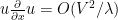
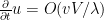
Now we model the motion of water inside the ocean by assigning at each time 

We make the basic assumption of incompressibility, so that the density 

The velocity changes over time according to Newton’s second law 


Because of incompressibility, the area 


which simplifies to the incompressible Euler equation

At present, the pressure is not given. However, we can simplify things by making the assumption of (vertical) hydrostatic equilibrium, i.e. the vertical effect 


This reflects the intuitively plausible fact that the pressure at a point under the ocean should be determined by the weight of the water above that point.
The incompressible Euler equation now simplifies to

We next make the shallow water approximation that the wavelength of the water is far greater than the depth of the water. In particular, we do not expect significant changes in the velocity field in the

(This ansatz should be taken with a grain of salt, particularly when applied to the 

Taking the 

The next step is to play off the incompressibility of water against the finite depth of the ocean. Consider an infinitesimal slice

of the ocean at some time 

and so the rate of change of mass of this slice over time is

On the other hand, the rate of mass entering this slice on the left 

and the rate of mass exiting on the right 

Putting these three facts together, we obtain the equation


which simplifies after Taylor expansion to the second shallow water wave equation

Remark 1 Another way to derive (7) is to use a more familiar form of the incompressibility, namely the divergence-free equation
(Here we will refrain from applying (5) to the vertical component of the velocity
at the surface of the ocean, we have the formulae
and
which after application of the chain rule gives the equation
A similar analysis at the ocean floor (which does not vary in time) gives
We apply these equations to the evaluation of the expression
which is the spatial rate of change of the velocity flux through a vertical slice of the ocean. On the one hand, using the ansatz (5), we expect this expression to be approximately
On the other hand, by differentiation under the integral sign, we can evaluate this expression instead as
If we then substitute in (8), (9), (10) and apply the fundamental theorem of calculus, one ends up with
, and the claim (7) follows.


The equations (6), (7) are nonlinear in the unknowns 

This hypothesis is fairly accurate for tsunamis in the deep ocean, and even for medium depths, but of course is not reasonable once the tsunami has reached shore (where the dynamics are far more difficult to model).
The hypothesis (11) already simplifies (7) to (approximately)

As for (6), we argue that the second term on the left-hand side is negligible, leading to

To explain heuristically why we expect this to be the case, let us make the ansatz that 


and equation (12) then suggests

From (11) we expect 

If we now insert the above ansatz into (13), we obtain

combining this with (14), we already get the velocity relationship (1).
Remark 2 One can also obtain (1) more quickly (up to a loss of a constant factor) by dimensional analysis, together with some additional physical arguments. Indeed, it is clear from a superficial scan of the above discussion that the velocity
. As the density
, we expect the wavelength to be physically undetectable at local scales (it requires not only knowledge of the slope of the height function at one’s location, but also the second derivative of that function (i.e. the curvature of the ocean surface), which is lower order). So we rule out dependence on
and
To get the relation (2), we have to analyse the ansatz a bit more carefully. First, we combine (13) and (12) into a single equation for the height function

To solve this wave equation, we use a standard sinusoidal ansatz

where 


and the Hamilton-Jacobi equation

From the eikonal equation we see that 

As for the Hamilton-Jacobi equation, we solve it using the method of characteristics. Multiplying the equation by

Inserting (15) and writing 

which simplifies to

Thus we see that 

so 


which gives (2).
Remark 3 It becomes difficult to retain the sinusoidal ansatz once the amplitude exceeds the depth, as it leads to the absurd conclusion that the troughs of the wave lie below the ocean floor. However, a remnant of this effect can actually be seen in real-life tsunamis, namely that if the tsunami starts with a trough rather than a crest, then the water at the shore draws back at first (sometimes for hundreds of metres), before the crest of the tsunami hits. As such, the sudden withdrawal of water of a shore is an important warning sign of an immediate tsunami.

35 comments
Comments feed for this article
13 March, 2011 at 10:39 pm
Pencil
Thanks for the article. Good night!
13 March, 2011 at 10:54 pm
daf
This is nothing original. Go and predict an earthquake if you can.
14 March, 2011 at 9:40 am
shortstop
Yes, one finds shallow water equation and its application from fluid mechanics textbooks. I believe he puts here just for educational purposes and meanwhile He never said that’s an original work. You needn’t so offensive. Just be polite, please. BTW, he tried to describe tsunami and you mentioned earthquake which is totally different natural phenomena though the latter can cause the former.
15 March, 2011 at 5:28 pm
Anonymous
it’s obvious where the down vote came from:)
13 March, 2011 at 11:44 pm
Rod Carvalho
Shouldn’t it be instead of
  ?
?
[Fixed, thanks – T.]
14 March, 2011 at 5:11 am
math dictionary
Nice.
Even the tsunami have so much details of mathematics.
I hope one day math and science will be able to predict tsunami before it comes.
5 July, 2013 at 9:31 pm
Laurence
The Occurrence of Tsunami is hard to predict but since the cause can be determined, it can be known when the waves will arrive at the shore. I can make a better paper than this. You wait… his article is too nerdy but can be appreciated. I look in my book when I was just a kid, I saw ocean mapping being done by scientist. With development of certain technology we may know when the waves will come to the shoreline and when we can counter it. The force of water can be displaced…This is certain. So displacing the initial force that would cause a great wave to the shore is crucial.
14 March, 2011 at 10:10 am
mathematicsnonentity
Now here is what I want to know:Are Tsunamis solitons…quasi solitons ..if there is such a thing?
If the answer to the above is yes, does any of the mathematics in professors Tao’s post relate-in a nontrivial way to the KDV-equations and the hierarchy equations in general.
14 March, 2011 at 10:33 am
Terence Tao
Well, solitons are large-amplitude (and thus nonlinear) phenomena, whereas tsunami propagation (in deep water, at least) is governed by low-amplitude (and thus essentially linear) equations. Typically, linear waves disperse due to the fact that the group velocity is usually sensitive to the wavelength; but in the tsunami regime, the group velocity is driven by pressure effects that relate to the depth of the ocean rather than the wavelength of the wave, and as such there is essentially no dispersion, thus creating traveling waves that have some superficial resemblance to solitons, but arise through a different mechanism.
It is true, though, that KdV also arises from a shallow water wave approximation. The main distinction seems to be that the shallow water equation comes from assuming that the pressure behaves like the hydrostatic pressure, whereas KdV arises if one assumes instead that the velocity is irrotational (which is definitely not the case for tsunami waves).
29 March, 2011 at 12:02 pm
Tony Roberts
I suspect that this answer may mislead. First, are tsunamis solitons? the answer depends how rigorous you want to be. Theoretically we do not know whether real tsunamis are true solitons. However, some of the video footage of the tsunami approaching Japan’s shore certainly show waves that I would like to call solitons. Further, classic approximate models like KdV or shallow water models also give soliton-like solutions. Might as well call them solitons then. Except it also depends upon initial conditions and the shoaling of the waves.
Do they arise through different mechanisms? I would not say so either. In classic scattering theory, solitons emerge from general compact disturbances (such as the local earthquake), but work also shows they emerge in shoaling, so the appearance of soliton-like waves on Japan’s shore looks like standard mechanisms at work.
On the distinction between KdV and shallow water waves: the classic derivation of the KdV for water waves is to take the shallow water wave equation and assume waves are only propagating in one direction. Thus the KdV is simply a restriction of shallow water wave equation and shares all its approximations, plus one more.
Finally, on a related but different issue: it strikes me as incongruous that our modelling for floods, tides, and tsunamis is based upon smooth, inviscid, irrotational flow when one can plainly see viscous turbulence in the flows. I have tried intermittently to base shallow water models on turbulent models, but it is difficult.
14 March, 2011 at 11:02 am
mathematicsnonentity
Professor Tao
Historical note:Korteweg and deVries famous equation was published a few months before the 1896 Tsunami that struck Japan killing thirty thousand Japanese.
The speed of propagation equation of a Tsunami is the same as the average speed of a Soliton…I think?
14 March, 2011 at 5:04 pm
ViceRoy
Thx for information.
I’m studying Physical Oceanography in South Korea – near by Japan.
15 March, 2011 at 6:34 am
ETH Alumni Math • Phys » Mathematics and Tsunami Propagation
[…] Nach den tragischen Ereignissen in Japan hat Terence Tao, Empfänger der Fields-Medaille 2006, einen Blogeintrag zur Fortbewegung von Tsunami-Wellen veröffentlicht. Die Mathematik und Physik der zerstörerischen Welle werden hauptsächlich durch hyperbolische partielle Differentialgleichungen, die sogenannten “shallow water equations”, und “wave shoaling” beschrieben. Den ausführlichen Eintrag findet ihr hier. […]
15 March, 2011 at 9:52 am
MSRI Workshop Day 2 (a week later!): Free boundary problems involving thin films «
[…] Bertozzi. Incidentally, Terry Tao discussed the closely related shallow water wave equation in a blog plost […]
16 March, 2011 at 2:29 pm
Helal
It is a nice article, and thanks to professor Tao.
As we know, the KdV under some initial conditions leads to the solitons. But the accurate mathematical model that describe the Tsunamis need more and more justifications. What do you think?!
17 March, 2011 at 11:20 pm
Tsunami « UGroh's Weblog
[…] Tsunami-Welle ist schon viel berichtet worden. Wer es genau wissen will, den möchte ich auf den Artikel auf dem Blog von Terence Tao hinweisen. Wer ist nicht so genau wissen will, aber dennoch sein Allgemeinwissen bereichern […]
19 March, 2011 at 11:37 am
State of Technology Last Week -#3 « Dr Data's Blog
[…] Serious Reading – Math of Tsunami vs. shallow wave propagation […]
23 March, 2011 at 3:07 pm
Anonymous
Wonderful article. Never imagine there is so much math behind waves. Now I am wondering if there are any deep math theories behind earthquakes?
26 March, 2011 at 10:30 am
Second Xamuel.com Linkfest
[…] Terence Tao: Bezout’s inequality, The shallow water wave equation and tsunami propagation […]
26 March, 2011 at 1:35 pm
Happenings – 2011 Mar 26 « Rip’s Applied Mathematics Blog
[…] has a derivation of the tsunami wave equation – that is, of the equation we use for tsunamis until they get close to […]
28 September, 2011 at 6:30 am
petequinn
I had forgotten about this interesting article, but recently attended a very interesting lecture by a noted engineer who studied under Japanese researchers and who studies tsunamis. His presentation included some excellent graphics (photos and plenty of video) from this year’s disastrous tsunami in Japan, and also made frequent reference to the mid-2000s tsunami disaster.
I gather the tsunami, once it crashes on shore, no longer behaves like a wave at all, but rather changes to a moving bore of turbulent flow. In the presentation, the speaker emphasized that modern models tend to be wildly inaccurate at predicting the run-up height of tsunamis. Models applied to the Japan tsunami tended to be off by up to about 15 m between actual and predicted run-up height.
I don’t recall much about fluid dynamics, but I think I understood the turbulent flow is a mathematically intractable problem, and I also recall that this was one of the early problems Mandelbrot applied his new fractal geometry to. Can anyone point me to successful applications of fractal-based analysis of this or similar chaotic physical problems?
6 December, 2011 at 3:04 pm
dlw
(2) is erroneous. It should be:
Wave amplitude A is proportional to 1/sqrt(sqrt(b)), where b is the water depth.
This is the so-called Green’s Law, derived by George Green in 1837.
(Green, Cambridge Trans. VI, 457, 1837).
Here is a heuristic proof via energy conservation:
The wave energy E within a wavelength is proportional to A^2 * L,
where A is the wave amplitude, L the wave length (Lambda in the blog), which is proportional to the wave speed v, which in turn, is proportional to sqrt(b). Thus the energy E is proportional to A^2*sqrt(b). Energy conservation (as the wave propagates) dictates:
A^2*sqrt(b) = C, where C is a constant
Thus,
A = C/sqrt(sqrt(b)) (G)
This is the so-called Green’s Law
The increase of wave amplitude as the waves approach the shore is still dramatic
but as not as dramatic as described by (2).
According to (2): 1-m wave in 5000 m deep water would be 22 m in 10 m water. According to the Green’s law (G), 1-m wave in 5000 m deep water would be about 5 m
in 10 m water.
6 December, 2011 at 4:43 pm
Terence Tao
Thanks for pointing out the error! It took me a while to track down what happened; eventually I found that I had assumed in the sinusoidal ansatz that the velocity and height functions were perfectly in phase, which is of course incorrect. I’ve repaired the calculation now (working with a single second-order wave equation for the height, rather than a coupled first-order system for velocity and height, as I seem to make fewer mistakes with scalar equations than with systems).
14 March, 2012 at 3:53 pm
R J Green
“The sweep of long water waves across the Pacific”
Australian Journal of Physics., 14, 120-128, 1960.
provides a readable account of velocities of ‘ripples’ and ‘tuunamis’ , and the method of predicting the arrival time of the Tsuname; Chile to Sudney (Aust).
25 July, 2012 at 4:22 am
Anonymous
Hello, I do not understand any of this, as I am a high school student. I am doing a project on the application of trigonometry in tsunami wave analysis. i am aiming to find out the impact of waves on the coastline so tsunami waves can be predicted. I am in need of formulas to help me in this. Pls help me find some relevant formulas…anyone willing to help?
29 May, 2013 at 3:37 am
Laurence Edgardo A. del Puerto
no need to predict it… it is already a regular occasion. try focusing your mind on how to minimize its effects one its cause will trigger the tragedy.
4 December, 2016 at 11:33 pm
Trinity Curtis
I’m in 8th grade, and am doing a project similar to this, and I do have one equation that I believe would work quite well for determining the impact of a wave.
dM/dt=−14ρgA squared
While p represents water density, g is gravity, A is the height of the wave (middle to crest),and d represents the average water depth
this is the formula for momentum flux, with a negative downwards based on gravity.
wow this comment is from 2012. hope had a nice graduation
24 February, 2013 at 6:35 am
Pete Cadmus
Great article. Thanks for taking the time to post all this.
1 May, 2013 at 8:40 am
ocean | sea | Annotary
[…] Ferreira: physics complexity sustainability & energy biology Sort Share terrytao.wordpress.com 4 minutes […]
29 May, 2013 at 3:35 am
Laurence Edgardo A. del Puerto
Have you at least simulated a tsunami effect in an aquarium before you made this article? I would have if only some one will fund my project and ultimately can find a way to counter it. I bet my life on it that I could figure a way to at least minimize its effects if not on the first or second wave… then maybe on the third wave.
26 September, 2014 at 4:08 am
My great WordPress blog – Econlinks: The applied maths edition
[…] wave equation and tsunami propagation: a concise exposition by Terry Tao. Brings back nice memories of my maths classes at Utrecht […]
22 September, 2015 at 10:29 am
Everything You Need to Know to Survive a Tsunami - FunaGram
[…] floor. In some ways, this is fantastic: the fluid dynamics of shallow-water waves make it extremely easy to predict tsunami travel times[7], and thus when the waves will start arriving on distant shores. On the down side, it’s […]
18 January, 2017 at 7:09 pm
Anonymous
I’m doing a science fair project about how wave depth affects wave velocity on tsunamis. I have to cite it but I don’t see a citations pg. By any chance you could put one next time. Thanks
17 July, 2017 at 3:42 am
Tsunamier: Store bølger med katastrofale følger – Ekte data
[…] https://terrytao.wordpress.com/2011/03/13/the-shallow-water-wave-equation-and-tsunami-propagation/#p… […]
10 January, 2024 at 12:45 am
Anonymous
A small typo – In Remark 2, “and which is negligible when compared against the phase velocity V”, V should be v.
[Corrected, thanks – T.]