
Hilbert’s fifth problem concerns the minimal hypotheses one needs to place on a topological group 


for sufficiently small 

We now reduce the regularity hypothesis further, to one in which there is no explicit Euclidean space that is initially attached to
Lemma 1 If
), and
is a linear subspace of
We will establish a non-linear version of this statement, known as Cartan’s theorem. Recall that a subset 


Theorem 2 (Cartan’s theorem) If
is a (topologically) closed subgroup of a Lie group
Note that the hypothesis that 

Exercise 1 Let
A variant of the above results is provided by using (faithful) representations instead of embeddings. Again, the linear version is trivial:
Lemma 3 If
from
Here is the non-linear version:
Theorem 4 (von Neumann’s theorem) If
, then
Actually, it will suffice for the homomorphism 
Example 1 Let
be the two-dimensional torus, let
, and let
, where
is a fixed real number. Then
is irrational, and so Theorem 4 is consistent with the fact that
is not closed; and so Theorem 4 does not follow immediately from Theorem 2 in this case. (We will see, though, that Theorem 4 follows from a local version of Theorem 2.)
As a corollary of Theorem 4, we observe that any locally compact Hausdorff group 

In all of these cases, one is not really building up Euclidean or Lie structure completely from scratch, because there is already a Euclidean or Lie structure present in another object in the hypotheses. Now we turn to results that can create such structure assuming only what is ostensibly a weaker amount of structure. In the linear case, one example of this is is the following classical result in the theory of topological vector spaces.
Theorem 5 Let
Remark 1 The Banach-Alaoglu theorem asserts that in a normed vector space
is always compact in the weak-* topology. Of course, this dual space
The full non-linear analogue of this theorem would be the Gleason-Yamabe theorem, which we are not yet ready to prove in this set of notes. However, by using methods similar to that used to prove Cartan’s theorem and von Neumann’s theorem, one can obtain a partial non-linear analogue which requires an additional hypothesis of a special type of metric, which we will call a Gleason metric:
Definition 6 Let
which generates the topology on
, writing
for
:
- (Escape property) If
and
is such that
, then
.
- (Commutator estimate) If
are such that
, then
where
is the commutator of
and
.
![\displaystyle \|[g,h]\| \leq C \|g\| \|h\|, \ \ \ \ \ (1)](https://s0.wp.com/latex.php?latex=%5Cdisplaystyle++%5C%7C%5Bg%2Ch%5D%5C%7C+%5Cleq+C+%5C%7Cg%5C%7C+%5C%7Ch%5C%7C%2C+%5C+%5C+%5C+%5C+%5C+%281%29&bg=ffffff&fg=000000&s=0&c=20201002)
Exercise 2 Let
Theorem 7 (Building Lie structure from Gleason metrics) Let
We will rely on Theorem 7 to solve Hilbert’s fifth problem; this theorem reduces the task of establishing Lie structure on a locally compact group to that of building a metric with suitable properties. Thus, much of the remainder of the solution of Hilbert’s fifth problem will now be focused on the problem of how to construct good metrics on a locally compact group.
In all of the above results, a key idea is to use one-parameter subgroups to convert from the nonlinear setting to the linear setting. Recall from the previous notes that in a Lie group 
Exercise 3 The purpose of this exercise is to illustrate the perspective that a topological group can be viewed as a non-linear analogue of a vector space. Let
be locally compact groups. For technical reasons we assume that
-compact and metrisable.
- (i) (Open mapping theorem) Show that if
is a continuous homomorphism which is surjective, then it is open (i.e. the image of open sets is open). (Hint: mimic the proof of the open mapping theorem for Banach spaces, as discussed for instance in these notes. In particular, take advantage of the Baire category theorem.)
- (ii) (Closed graph theorem) Show that if a homomorphism
is a closed subset of
), then it is continuous. (Hint: mimic the derivation of the closed graph theorem from the open mapping theorem in the Banach space case, as again discussed in these notes.)
- (iii) Let
be a continuous injective homomorphism into another Hausdorff topological group
. Show that
is continuous if and only if
is continuous.
- (iv) Relax the condition of metrisability to that of being Hausdorff. (Hint: Now one cannot use the Baire category theorem for metric spaces; but there is an analogue of this theorem for locally compact Hausdorff spaces.)
— 1. The theorems of Cartan and von Neumann —
We now turn to the proof of Cartan’s theorem. As indicated in the introduction, the fundamental concept here will be that of a one-parameter subgroup:
Definition 8 (One-parameter subgroups) Let
. The space of all such one-parameter subgroups is denoted
.
Remark 2 Strictly speaking, the terminology “one-parameter subgroup” is a misnomer, because it is the image
of
of a one-parameter subgroup
, where
is a non-zero real number, to be distinct from
, even though both one-parameter subgroups have the same image.
We recall Exercise 12 from the previous set of notes, which we reformulate here as a lemma:
Lemma 9 (Classification of one-parameter subgroups) Let
is an element of
is a one-parameter subgroup; conversely, if
such that
for all
. Thus we have a canonical one-to-one correspondence between
Now let

Thus we can think of 


We claim that 


Since 


The next step is to show that
Lemma 10 Suppose that the identity
is not an isolated point of
Proof: As 


Let us arbitrarily endow the finite-dimensional vector space 

Let 


Now we establish a stronger version of the above lemma:
Lemma 11 There exists a neighbourhood
is a homeomorphism.
Proof: Let 


As 


We arbitrarily place a norm on 

Since 


From the above lemma we see that 

Remark 3 Observe a posteriori that
There is a local version of Cartan’s theorem, in which groups are replaced by local groups:
Theorem 12 (Local Cartan’s theorem) If
of the identity in
The proof of this theorem follows the lines of the global Cartan’s theorem, with some minor technical changes, and we set this proof out in the following exercise.
Exercise 4 Define a local one-parameter subgroup of a local group
from the (additive) local group
to
- (i) If
- (ii) In the situation of Theorem 12, show that
- (iii) Let the notation and assumptions be as in (ii). For any neighbourhood
.
- (iv) Let the notation and assumptions be as in (ii). There exists a neighbourhood
- (v) Prove Theorem 12.

One can then use Theorem 12 to establish von Neumann’s theorem, as follows. Suppose that 


Remark 4 State and prove a local version of von Neumann’s theorem, in which
— 2. Locally compact vector spaces —
We will now turn to the study of topological vector spaces, which we will need to establish Theorem 7. We begin by recalling the definition of a topological vector space.
Definition 13 (Topological vector space) A topological vector space is a (real) vector space
and
(jointly) continuous. (In particular,
is necessarily a topological group.)
One can also consider complex topological vector spaces, but the theory for such spaces is almost identical to the real case, and we will only need the real case for what follows. In the literature, it is often common to restrict attention to Hausdorff topological vector spaces, although this is not a severe restriction in practice, as the following exercise shows:
Exercise 5 Let
of the origin is a closed subspace of
is a Hausdorff topological vector space. Furthermore, show that a set is open in
.
An important class of topological vector spaces are the normed vector spaces, in which the topology is generated by a norm 
We emphasise that in order to be a topological vector space, the vector space operations 
Example 2 Consider the one-dimensional vector space
space (though not Hausdorff), the scalar multiplication map
is jointly continuous, and the addition map
is continuous in each coordinate (i.e. translations are continuous), but not jointly continuous; for instance, the set
does not contain a non-trivial Cartesian product of two sets that are open in the co-compact topology. So this is not a topological vector space. Similarly for the cocountable or cofinite topologies on
Example 3 Consider the topology of
. This pullback topology is not quite Hausdorff, but the addition map
under the map
for some irrational
Example 4 Consider
These examples illustrate that a vector space such as
Theorem 14 Every finite-dimensional Hausdorff topological vector space has the usual topology.
Proof: Let 
Let 


is continuous. From this, we see that any set which is open in
Now we show conversely that every set which is open in the usual topology, is open in
We use 


At present, 


We isolate one important consequence of the above theorem:
Corollary 15 In a Hausdorff topological space
Proof: It suffices to show that every vector 
We can now prove Theorem 5. Let 

for some finite set

Iterating this we have
for any 


for any neighbourhood

But 

Exercise 6 Establish the Riesz lemma: if
is a normed vector space,
, then there exists a vector
and
. (Hint: pick an element
of
that nearly minimises
. Use these two vectors to construct a suitable
— 3. From Gleason metrics to Lie groups —
Now we prove Theorem 7. The argument will broadly follow the lines of Cartan’s theorem, but we will have to work harder in many stages of the argument in order to compensate for the lack of an obvious ambient Lie structure in the initial hypotheses. In particular, the Gleason metric hypothesis will substitute for the
Henceforth, 
We use the asymptotic notation 


Note that the left-invariant metric properties of

and the triangle inequality

From the commutator estimate (1) and the triangle inequality we also obtain a conjugation estimate

whenever 
we then conclude an approximate right invariance
whenever 

whenever
This has the following useful consequence, which asserts that the power maps 
and
 , then

Proof: We begin with the first inequality. By the triangle inequality, it suffices to show that

uniformly for all 

which by (2) is bounded above by

as required.
Now we prove the second estimate. Write 


thanks to the escape property (shrinking 

If
Remark 5 Lemma 16 implies (by a standard covering argument) that the group
Now we bring in the space

for 


![{[-1,1]}](https://s0.wp.com/latex.php?latex=%7B%5B-1%2C1%5D%7D&bg=ffffff&fg=000000&s=0&c=20201002)
Given that
Lemma 17
Proof: It is easy to see that 
![{I = [-T,T]}](https://s0.wp.com/latex.php?latex=%7BI+%3D+%5B-T%2CT%5D%7D&bg=ffffff&fg=000000&s=0&c=20201002)

![{t \in [-T,T]}](https://s0.wp.com/latex.php?latex=%7Bt+%5Cin+%5B-T%2CT%5D%7D&bg=ffffff&fg=000000&s=0&c=20201002)
![\displaystyle B := \{ \phi \in L(G): \sup_{t \in [-T,T]} d(\phi(t),\phi_0(t)) < \epsilon \}](https://s0.wp.com/latex.php?latex=%5Cdisplaystyle++B+%3A%3D+%5C%7B+%5Cphi+%5Cin+L%28G%29%3A+%5Csup_%7Bt+%5Cin+%5B-T%2CT%5D%7D+d%28%5Cphi%28t%29%2C%5Cphi_0%28t%29%29+%3C+%5Cepsilon+%5C%7D&bg=ffffff&fg=000000&s=0&c=20201002)
is totally bounded. By the Arzelá-Ascoli theorem, it suffices to show that the family of functions in 
By construction, we have 


We observe for future reference that the proof of the above lemma also shows that all one-parameter subgroups are locally Lipschitz.
Now we put a vector space structure on 


which is easily seen to actually be a one-parameter subgroup.
Now we turn to the addition operation. In the Lie group case, one can express the one-parameter subgroup 


cf. Exercise 15 from the previous notes. In view of this, we would like to define the sum 


Proof: To show well-definedness, it suffices to show that for each 

as

Observe from continuity of multiplication that to prove this claim for a given 
Let 

for all

if 

if 
The above argument in fact shows that

and

for all 


and similarly for 


but 


Lemma 19
Proof: We first show that 


An inspection of the argument used to establish (18) reveals that there is a constant

for all small

(thanks to Lemma 16). Similarly we have (after adjusting

From Lemma 16 we have

and thus

Similarly for 

sending
Finally, we need to show that the vector space operations are continuous. It is easy to see that scalar multiplication is continuous, as are the translation operations; the only remaining thing to verify is that addition is continuous at the origin. Thus, for every 
![{\sup_{t \in [-1,1]} \| (\phi+\psi)(t) \| \leq \epsilon}](https://s0.wp.com/latex.php?latex=%7B%5Csup_%7Bt+%5Cin+%5B-1%2C1%5D%7D+%5C%7C+%28%5Cphi%2B%5Cpsi%29%28t%29+%5C%7C+%5Cleq+%5Cepsilon%7D&bg=ffffff&fg=000000&s=0&c=20201002)
![{\sup_{t \in [-1,1]} \| \phi(t) \| \leq \delta}](https://s0.wp.com/latex.php?latex=%7B%5Csup_%7Bt+%5Cin+%5B-1%2C1%5D%7D+%5C%7C+%5Cphi%28t%29+%5C%7C+%5Cleq+%5Cdelta%7D&bg=ffffff&fg=000000&s=0&c=20201002)
![{\sup_{t \in [-1,1]} \| \psi(t) \| \leq \delta}](https://s0.wp.com/latex.php?latex=%7B%5Csup_%7Bt+%5Cin+%5B-1%2C1%5D%7D+%5C%7C+%5Cpsi%28t%29+%5C%7C+%5Cleq+%5Cdelta%7D&bg=ffffff&fg=000000&s=0&c=20201002)


![{t \in [-1,1]}](https://s0.wp.com/latex.php?latex=%7Bt+%5Cin+%5B-1%2C1%5D%7D&bg=ffffff&fg=000000&s=0&c=20201002)

Exercise 7 Show that for any
exists and defines a norm on

As
In analogy with the Lie algebra setting, we define the exponential map 

Exercise 8 Show that the exponential map is locally injective near the origin. (Hint: from Lemma 16, obtain the unique square roots property: if
, then
.)
We have proved a number of useful things about
Proposition 20 Suppose that
Of course, the converse is obvious; discrete groups do not admit any non-trivial one-parameter subgroups.
Proof: As 


We define the approximate one-parameter subgroups ![{\phi_n: [-1,1] \rightarrow G}](https://s0.wp.com/latex.php?latex=%7B%5Cphi_n%3A+%5B-1%2C1%5D+%5Crightarrow+G%7D&bg=ffffff&fg=000000&s=0&c=20201002)
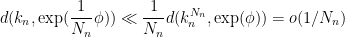
Then we have 


uniformly whenever 

![{\phi: [-1,1] \rightarrow G}](https://s0.wp.com/latex.php?latex=%7B%5Cphi%3A+%5B-1%2C1%5D+%5Crightarrow+G%7D&bg=ffffff&fg=000000&s=0&c=20201002)


We now generalise the above proposition to a more useful result (cf. Lemma 11).
Proposition 21 For any neighbourhood
is a neighbourhood of the identity in
Proof: We use an argument of Hirschfeld (communicated to me by van den Dries and Goldbring). By shrinking
Suppose for contradiction that 


and hence 
Let 

Let
As before, we may pass to a subsequence such that
In a similar vein, since 


We now claim that 

Since 

But from Lemma 16 again, one has
and thus
But for 

If 

Exercise 9 If we identify
Proposition 22
Proof: The radial homogeneity is clear from (4) and the homomorphism property, so the main task is to establish the
for the local group law

for

for all 

Combining this proposition with Lemma 16 from the previous notes, we obtain Theorem 7.
Exercise 10 State and prove a version of Theorem 7 for local groups. (In order to do this, you must first decide how to define an analogue of a Gleason metric on a local group.)

14 comments
Comments feed for this article
11 September, 2011 at 3:07 pm
David Roberts
The last sentence of the first paragraph should be ‘we call such local groups…’.
Also, the sentence ‘the one-parameter subgroups are in one-to-one correspondence with the Lie algebra g’ doesn’t make sense. Do you mean ‘elements of the Lie algebra g’?
[Corrected, thanks – T.]
27 September, 2011 at 3:30 pm
254A, Notes 3: Haar measure and the Peter-Weyl theorem « What’s new
[…] the last few notes, we have been steadily reducing the amount of regularity needed on a topological group in order to […]
4 October, 2011 at 12:58 pm
254A, Notes 4: Building metrics on groups, and the Gleason-Yamabe theorem « What’s new
[…] Gleason-Yamabe theorem, we will use three major tools developed in previous notes. The first (from Notes 2) is a criterion for Lie structure in terms of a special type of metric, which we will call a […]
8 October, 2011 at 12:58 pm
254A, Notes 5: The structure of locally compact groups, and Hilbert’s fifth problem « What’s new
[…] to the quotient of by a compact normal subgroup . By Cartan’s theorem (Theorem 2 of Notes 2), is also a Lie group. Among other things, this implies that the quotient homomorphism from the […]
9 October, 2011 at 7:03 am
pavel zorin
Dear Prof. Tao,
In the proof of theorem 14 one can use the continuity of scalar multiplication at (0,0) to make U bounded. This is easier and also shows that the continuity of addition is not needed in this step.
best regards,
pavel
[Good point; I’ve made the change. -T.]
16 October, 2011 at 10:26 am
Ben Hayes
In Lemma 17 I don’t quite see how you apply the escape property. To apply the escape property, you need to already know that whereas it appears that at this stage you only know
16 October, 2011 at 2:51 pm
Terence Tao
If exceeds 1/C, then one works instead with the largest positive integer m for which
  ; this will be an integer between 1 and n, and for
  small enough one can show that one must have
  to avoid a contradiction.
(More generally, one often encounters “almost circular reasoning” issues in these sorts of problems, in which one almost has to assume the result one is trying to prove as a hypothesis. Often, one has to deal with the apparent circularity by an induction argument, a bootstrap argument, a continuity argument, an infinite descent argument, or passing to the “first counterexample” or “last example”. The above is an instance of the latter strategy.)
16 October, 2011 at 4:43 pm
Ben Hayes
Ah, when I go through the estimates I see the contradiction now. Thanks.
27 October, 2011 at 8:37 pm
254A, Notes 7: Models of ultra approximate groups « What’s new
[…] create a metric structure on strong approximate groups analogous to the Gleason metrics studied in previous notes, which can in turn be exploited (together with an induction on dimension argument) to fully […]
1 December, 2011 at 7:58 am
254A, Notes 8: The microstructure of approximate groups « What’s new
[…] was a key difficulty in the theory surrounding Hilbert’s fifth problem that was discussed in previous notes. A key tool in being able to resolve such structure was to build left-invariant metrics (or […]
20 November, 2012 at 6:31 pm
The closed graph theorem in various categories « What’s new
[…] There is also a number of closed graph theorems for topological groups, of which the following is typical (see Exercise 3 of these previous blog notes): […]
5 September, 2013 at 9:23 pm
Notes on simple groups of Lie type | What's new
[…] complex Lie group but are clearly not a Lie group. However, a basic theorem of Cartan (proven in this previous post) says that any subgroup of a real Lie group which is topologically closed, is also a real Lie […]
21 December, 2018 at 4:30 am
Piotr
Dear Professor Tao!
For a few months I’m deeply studying your book about Hilbert’s Fifth Problem. I stacked in Exercise 9 (formulated above on the web page), which is crucial in the proof of Proposition 22. One of Lipschitz conditions in Exercise 9 is equivalent to the following:
If (in a NSS group with Gleason metric):
n ||g|| < A and n ||h|| < A (for sufficiently small A), then:
||(gh)^n|| < B ||g^n h^n|| (for sufficiently large, but fixed, B)
I have no idea how to show this property! I spent many hours on this and finally gave up. Thus, I'd kindly like to ask you about any hint to show that the inverse of exp is Lipschitz in a small neighbourhood of the unit of G.
Thanks in advance for your help.
21 December, 2018 at 2:16 pm
Piotr
OK, got it – it is hidden in the proof of Lemma 16.