
In this set of notes, we describe the basic analytic structure theory of Lie groups, by relating them to the simpler concept of a Lie algebra. Roughly speaking, the Lie algebra encodes the “infinitesimal” structure of a Lie group, but is a simpler object, being a vector space rather than a nonlinear manifold. Nevertheless, thanks to the fundamental theorems of Lie, the Lie algebra can be used to reconstruct the Lie group (at a local level, at least), by means of the exponential map and the Baker-Campbell-Hausdorff formula. As such, the local theory of Lie groups is completely described (in principle, at least) by the theory of Lie algebras, which leads to a number of useful consequences, such as the following:
- (Local Lie implies Lie) A topological group
is Lie (i.e. it is isomorphic to a Lie group) if and only if it is locally Lie (i.e. the group operations are smooth near the origin).
- (Uniqueness of Lie structure) A topological group has at most one smooth structure on it that makes it Lie.
- (Weak regularity implies strong regularity, I) Lie groups are automatically real analytic. (In fact one only needs a “local
” regularity on the group structure to obtain real analyticity.)
- (Weak regularity implies strong regularity, II) A continuous homomorphism from one Lie group to another is automatically smooth (and real analytic).
The connection between Lie groups and Lie algebras also highlights the role of one-parameter subgroups of a topological group, which will play a central role in the solution of Hilbert’s fifth problem.
We note that there is also a very important algebraic structure theory of Lie groups and Lie algebras, in which the Lie algebra is split into solvable and semisimple components, with the latter being decomposed further into simple components, which can then be completely classified using Dynkin diagrams. This classification is of fundamental importance in many areas of mathematics (e.g. representation theory, arithmetic geometry, and group theory), and many of the deeper facts about Lie groups and Lie algebras are proven via this classification (although in such cases it can be of interest to also find alternate proofs that avoid the classification). However, it turns out that we will not need this theory in this course, and so we will not discuss it further here (though it can of course be found in any graduate text on Lie groups and Lie algebras).
— 1. Local groups —
The connection between Lie groups and Lie algebras will be local in nature – the only portion of the Lie group that will be of importance will be the portion that is close to the group identity 
Definition 1 (Local group) A local topological group
, or local group for short, is a topological space
, a partially defined but continuous multiplication operation
for some domain
, and a partially defined but continuous inversion operation
, where
, obeying the following axioms:
- (Local closure)
is an open neighbourhood of
, and
is an open neighbourhood of
- (Local associativity) If
are such that
and
are both well-defined in
- (Identity) For all
,
.
- (Local inverse) If
is well-defined in
. (In particular this, together with the other axioms, forces
.)
We will sometimes use additive notation for local groups if the groups are locally abelian (thus if
is defined, then
is also defined and equal to
A local group is said to be symmetric if
, i.e. if every element
in
A local Lie group is a local group that is also a smooth manifold, in such a fashion that the partially defined group operations
are smooth on their domain of definition.
Clearly, every topological group is a local group, and every Lie group is a local Lie group. We will sometimes refer to the former concepts as global topological groups and global Lie groups in order to distinguish them from their local counterparts. One could also consider local discrete groups, in which the topological structure is just the discrete topology, but we will not need to study such objects in this course.
A model class of examples of a local (Lie) group comes from restricting a global (Lie) group to an open neighbourhood of the identity. Let us formalise this concept:
Definition 2 (Restriction) If
is an open neighbourhood of the identity in
of
and
, and with the group operations
,
respectively. If
), then this restriction
Thus, for instance, one can take the Euclidean space 


It is natural to ask the question as to whether every local group arises as the restriction of a global group. The answer to this question is somewhat complicated, and can be summarised as “essentially yes in certain circumstances, but not in general”. See this previous blog post for more discussion.
A key example of a local Lie group for this blog post will come from pushing forward a Lie group via a coordinate chart near the origin:
Example 1 Let
, and let
be a smooth coordinate chart from a neighbourhood
of the origin
maps
which is the set
defined by the formula
defined whenever
are well-defined and lie in
defined by the formula
defined whenever
are well-defined and lie in
is a local Lie group. We will sometimes denote this local Lie group as
, to distinguish it from the additive local Lie group
arising by restriction of
to

Example 2 Let
, and let
. If we then let
be the ball
and
, then
with
), and by the construction in the preceding exercise,
becomes a local Lie group with the operations
(defined whenever
all lie in
(defined whenever
and
both lie in
on
or
for such structures.


Many (though not all) of the familiar constructions in group theory can be generalised to the local setting, though often with some slight additional subtleties. We will not systematically do so here, but we give a single such generalisation for now:
Definition 3 (Homomorphism) A continuous homomorphism
between two local groups
is a continuous map from
with the following properties:
of
of
.
- If
is well-defined in
.
- If
are such that
is well-defined in
is well-defined and equal to
.
A smooth homomorphism
It is easy to see that the composition of two continuous homomorphisms is again a continuous homomorphism; this gives the class of local groups the structure of a category. Similarly, the class of local Lie groups with their smooth homomorphisms is also a category.
Note that homomorphisms on a local group
Example 3 With the notation of Example 1,
provides the inverse homomorphism.
Let us say that a word 


Exercise 1 (Iterating the associative law)
- Show that if a word
- Give an example of a word
, so try
. A small discrete local group will already suffice to give a counterexample; verifying the local group axioms are easier if one makes the domain of definition of the group operations as small as one can get away with while still having the counterexample.)
— 2. Some differential geometry —
To define the Lie algebra of a Lie group, we must first quickly recall some basic notions from differential geometry associated to smooth manifolds (which are not necessarily embedded in some larger Euclidean space, but instead exist intrinsically as abstract geometric structures). This requires a certain amount of abstract formalism in order to define things rigorously, though for the purposes of visualisation, it is more intuitive to view these concepts from a more informal geometric perspective.
We begin with the concept of the tangent space and related structures.
Definition 4 (Tangent space) Let
be a smooth
of
defined on an open interval
containing
, modulo the relation that two curves
are considered equivalent if they have the same derivative at
where
is a coordinate chart of
with
. One easily verifies that this gives
.
The space
of pairs
, where
is a tangent vector of
If
is a smooth map between two manifolds, we define the derivative map
to be the map defined by setting
for all continously differentiable curves
. We also write
for
, so that for each
is a map from
. One can easily verify that this latter map is linear. We observe the chain rule
for any smooth maps
. (Indeed, one can view the tangent operator
and the derivative operator
together as a single covariant functor from the category of smooth manifolds to itself, although we will not need to use this perspective here.)
Observe that if
may be identified with
. In particular, every coordinate chart
of
, which gives
-dimensional manifold.


Remark 1 Informally, one can think of a tangent vector
on
is infinitesimally small; a smooth map
. One can make this informal perspective rigorous by means of nonstandard analysis, but we will not do so here.
Once one has the notion of a tangent bundle, one can define the notion of a smooth vector field:
Definition 5 (Vector fields) A smooth vector field on
which is a right inverse for the projection map
, thus (by slight abuse of notation)
maps
for some
. The space of all smooth vector fields is denoted
. It is clearly a real vector space. In fact, it is a
-module: given a smooth vector field
and a smooth function
(i.e. a smooth map
), one can define the product
in the obvious manner:
, and one easily verifies the module axioms.
Given a smooth function
of
along
whenever
; one easily verifies that
is well-defined and is an element of

Remark 2 One can define
where
is the projection map to the second coordinate of
; one can also view
Remark 3 If
from
of
from several variable calculus. If however one wishes to perform several changes of variable, then the more intrinsically geometric (and “coordinate-free”) perspective outlined above can be more helpful.
There is a fundamental link between smooth vector fields and derivations of
Exercise 2 (Correspondence between smooth vector fields and derivations) Let
- If
is a derivation on the (real) algebra
for all
.
- Conversely, if
is a derivation on
.

We see from the above exercise that smooth vector fields can be interpreted as a purely algebraic construction associated to the real algebra
Exercise 3 (Commutator of derivations is a derivation) Let
be two derivations on an algebra
. Show that the commutator
is also a derivation on
From the preceding two exercises, we can define the Lie bracket ![{[X,Y]}](https://s0.wp.com/latex.php?latex=%7B%5BX%2CY%5D%7D&bg=ffffff&fg=000000&s=0&c=20201002)

![\displaystyle \nabla_{[X,Y]} := [\nabla_X, \nabla_Y].](https://s0.wp.com/latex.php?latex=%5Cdisplaystyle++%5Cnabla_%7B%5BX%2CY%5D%7D+%3A%3D+%5B%5Cnabla_X%2C+%5Cnabla_Y%5D.&bg=ffffff&fg=000000&s=0&c=20201002)
This gives the space
Definition 6 (Lie algebra) A (real) Lie algebra is a real vector space
which is anti-symmetric (thus
for all
, or equivalently
for all
) and obeys the Jacobi identity
for all
.
![\displaystyle [[X,Y],Z] + [[Y,Z],X] + [[Z,X],Y] = 0 \ \ \ \ \ (3)](https://s0.wp.com/latex.php?latex=%5Cdisplaystyle++%5B%5BX%2CY%5D%2CZ%5D+%2B+%5B%5BY%2CZ%5D%2CX%5D+%2B+%5B%5BZ%2CX%5D%2CY%5D+%3D+0+%5C+%5C+%5C+%5C+%5C+%283%29&bg=ffffff&fg=000000&s=0&c=20201002)
Exercise 4 If
— 3. The Lie algebra of a Lie group —
Let 


If 


Exercise 5 Let
- Show that for every element
.
- Show that the commutator
From the above exercise, we can identify the tangent space ![{[,]}](https://s0.wp.com/latex.php?latex=%7B%5B%2C%5D%7D&bg=ffffff&fg=000000&s=0&c=20201002)

Remark 4 Informally, an element
of the identity in the Lie group
; for more abstract Lie groups, one can still formalise things using nonstandard analysis, but we will not do so here.
Exercise 6
- Show that the Lie algebra
of the general linear group
of
complex matrices, with the Lie bracket
.
- Describe the Lie algebra
of the unitary group
.
- Describe the Lie algebra
of the special unitary group
.
- Describe the Lie algebra
of the orthogonal
.
- Describe the Lie algebra
of the special orthogonal
.
- Describe the Lie algebra of the Heisenberg group
.
Exercise 7 Let
at the identity element
of
creates a covariant functor from the category of Lie groups to the category of Lie algebras.)
We have seen that every global Lie group gives rise to a Lie algebra. One can also associate Lie algebras to local Lie groups as follows:
Exercise 8 Let
left-invariant if, for every
, where
is the left-multiplication map
, defined on the open set
(where we adopt the convention that
is shorthand for “
is well-defined and lies in
Remark 5 In the converse direction, it is also true that every finite-dimensional Lie algebra can be associated to either a local or a global Lie group; this is known as Lie’s third theorem. However, this theorem is somewhat tricky to prove (particularly if one wants to associate the Lie algebra with a global Lie group), requiring the non-trivial algebraic tool of Ado’s theorem (discussed in this previous blog post); see Exercise 21 below.
— 4. The exponential map —
The exponential map 


- (i)
is the differentiable map obeying the ODE
and the initial condition
.
- (ii)
and the initial condition
.
- (iii)
as
.
- (iv)
.
We will need to generalise this map to arbitrary Lie algebras and Lie groups. In the case of matrix Lie groups (and matrix Lie algebras), one can use the matrix exponential, which can be defined efficiently by modifying definition (iv) above, and which was already discussed in the previous set of notes. It is however difficult to use this definition for abstract Lie algebras and Lie groups. The definition based on (ii) will ultimately be the best one to use for the purposes of this course, but for foundational purposes (i) or (iii) is initially easier to work with. In most of the foundational literature on Lie groups and Lie algebras, one uses (i), in which case the existence and basic properties of the exponential map can be provided by the Picard existence theorem from the theory of ordinary differential equations. However, we will use (iii), because it relies less heavily on the smooth structure of the Lie group, and will therefore be more aligned with the spirit of Hilbert’s fifth problem (which seeks to minimise the reliance of smoothness hypotheses whenever possible). Actually, for minor technical reasons it is slightly more convenient to work with the limit of 

We turn to the details. It will be convenient to work in local coordinates, and for applications to Hilbert’s fifth problem it will be useful to “forget” almost all of the smooth structure. We make the following definition:
Definition 7 (
for all sufficiently small
notation can depend on

Example 4 Let
. Then, as explained in Example 1,
is a local Lie group with identity
From Taylor expansion (using the smoothness of
. Thus we see that every local Lie group generates a

Remark 6 In real analysis, a (locally)
on a domain
which is continuously differentiable (i.e. in the regularity class
), and whose first derivatives
are (locally) Lipschitz (i.e. in the regularity class
) the
of twice continuously differentiable functions, but much stronger than the class
for any
in the domain of

We now estimate various expressions in a
Exercise 9 Let
.
- (i) Show that there exists an
whenever
and
are such that
, and the implied constant is uniform in
. Here and in the sequel we adopt the convention that a statement such as (5) is automatically false unless all expressions in that statement are well-defined. (Hint: induct on
in order to ensure that such constants remain uniform in
under the same hypotheses as above.
- (ii) Show that one has
for
- (iii) Show that
for
, then express
as the product of
and
.)
- (iv) Show that
whenever
- (v) Show that
whenever
- (vi) Show that there exists an
such that
whenever
are such that
.
- (vii) Show that there exists an
for all
and
such that
, where
is the product of
copies of
, and
.
- (viii) Show that there exists an
for all
as the product of
by various powers of


We can now define the exponential map 

for any 
Exercise 10 Let
- (i) Show that if
. (Hint: use the previous exercise to estimate the distance between
and
.) Establish the additional estimate
- (ii) Show that if
is a smooth curve with
, and
- (iii) Show that for all sufficiently small
Conclude in particular that for
is a homeomorphism between
of the origin. (Hint: To show that
- Show that
for
and
with
sufficiently small. (Hint: first handle the case when
are dyadic numbers.)
- (iv) Show that for any sufficiently small
Then conclude the stronger estimate
- (v) Show that for any sufficiently small
(Hint: use the previous part, as well as (viii) of Exercise 9.)


Let us say that a

whenever 

Corollary 8 Every
Now we study the exponential map on global Lie groups. If 

whenever
Exercise 11 Let
- (i) Show that the exponential map is well-defined. (Hint: First handle the case when
- (ii) Show that for all
and
and
(Hint: again, begin with the case when
- (iii) Show that the exponential map is continuous.
- (iv) Show that for each
, the function
is the unique homomorphism from
with derivative equal to


Proposition 9 (Lie’s first theorem) Let
Proof: We begin with the smoothness. From the homomorphism property we see that

for all 


for some smooth function 

Now let 


Since

we see that the derivative of the exponential map at the origin is the identity map on

In view of this proposition, we see that given a vector space basis 

for sufficiently small 

Using exponential coordinates of the first kind, we see that we may identify a local piece 
Exercise 12 (Classification of one-parameter subgroups) Let
, show that the map
is a one-parameter subgroup. Conversely, if
for all
Proposition 10 (Weak regularity implies strong regularity) Let
be a continuous homomorphism. Then
is smooth.
Proof: Since 

for all 


and thus

We conclude that

Since 
This fact has a pleasant corollary:
Corollary 11 (Uniqueness of Lie structure) Any (global) topological group can be made into a Lie group in at most one manner. More precisely, given a topological group
Proof: Suppose for sake of contradiction that one could find two different smooth structures on 


Note that a general high-dimensional topological manifold may have more than one smooth structure, which may even be non-diffeomorphic to each other (as the example of exotic spheres demonstrates), so this corollary is not entirely vacuous.
Exercise 13 Let
. In other words, if
is another continuous homomorphism with
, then
. (Hint: first prove this in a small neighbourhood of the origin. What group does this neighbourhood generate?) What happens if
Exercise 14 (Weak regularity implies strong regularity, local version) Let
Exercise 15 (Local Lie implies Lie) Let
are smooth near the origin for any
— 5. The Baker-Campbell-Hausdorff formula —
We now study radially homogeneous
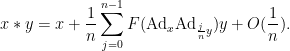
Theorem 12 (Baker-Campbell-Hausdorff formula, qualitative version) Let
be a radially homogeneous
We will in fact give a more precise formula for
Remark 7 In the case where
for sufficiently small
. Thus, a corollary of Theorem 12 is that this map is real analytic.
We begin the proof of Theorem 12. Throughout this section,
Exercise 16 (Lipschitz bounds) If
are sufficiently small, establish the bounds
(Hint: to prove (15), start with the identity
.)


Now we exploit the radial homogeneity to describe the conjugation operation 
Lemma 13 (Adjoint representation) For all
such that
for all
Remark 8 Using the matrix example from Remark 7, we are asserting here that
for some linear transform
of
for invertible
is a continuous ring homomorphism) we see that we may take
here.

Proof: Fix

for 
Let

Conjugating this by


But from (4) we have

and thus (by Exercise 16)

But if we split 


Putting all this together we see that


sending
From (4) we see that
for
for all

for 


for all sufficiently small 
From (21), (20), (4) we see that

for 
Also we clearly have 


![\displaystyle \hbox{ad}_x y = [x,y] \ \ \ \ \ (21)](https://s0.wp.com/latex.php?latex=%5Cdisplaystyle++%5Chbox%7Bad%7D_x+y+%3D+%5Bx%2Cy%5D+%5C+%5C+%5C+%5C+%5C+%2821%29&bg=ffffff&fg=000000&s=0&c=20201002)
for some bilinear form ![{[,]: {\bf R}^d \rightarrow {\bf R}^d}](https://s0.wp.com/latex.php?latex=%7B%5B%2C%5D%3A+%7B%5Cbf+R%7D%5Ed+%5Crightarrow+%7B%5Cbf+R%7D%5Ed%7D&bg=ffffff&fg=000000&s=0&c=20201002)
One can show that this bilinear form in fact defines a Lie bracket (i.e. it is anti-symmetric and obeys the Jacobi identity), but for now, all we need is that it is manifestly real analytic (since all bilinear forms are polynomial and thus analytic). In particular 
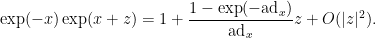
We now give an important approximation to 
Lemma 14 For
where


Proof: If we write 


We will shortly establish the approximation

inverting
we obtain the claim.
It remains to verify (22). Let

Using (11), the first summand can be expanded as

From (15) one has 

which by definition of 

From (15) one has
while from (20) one has 

Inserting this back into (23), we can thus write the left-hand side of (22) as

Writing 

and the claim follows.
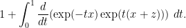
Remark 9 In the matrix case, the key computation is to show that
To see this, we can use the fundamental theorem of calculus to write the left-hand side as
Since
and
, we can rewrite this as
Since
, this becomes
since
, we obtain the desired claim.


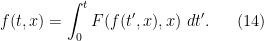
We can integrate the above formula to obtain an exact formula for
Corollary 15 (Baker-Campbell-Hausdorff-Dynkin formula) For

The right-hand side is clearly real analytic in
Proof: Let
From (11) followed by Lemma 14 and (21), one has


We conclude that
Sending
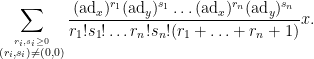
Exercise 17 Use the Taylor-type expansion
to obtain the explicit expansion
where
, and show that the series is absolutely convergent for


Exercise 18 Let
We now record some consequences of the Baker-Campbell-Hausdorff formula.
Exercise 19 (Lie groups are analytic) Let
Exercise 20 (Lie’s second theorem) Let
be a Lie algebra homomorphism. Show that there exists an open neighbourhood
from the local Lie group
. If
Exercise 21 (Lie’s third theorem) Ado’s theorem asserts that every finite-dimensional Lie algebra is isomorphic to a subalgebra of
for some
- (i) (Lie’s third theorem, local version) Every finite-dimensional Lie algebra is isomorphic to the Lie algebra of some local Lie group.
- (ii) Every local or global Lie group has a neighbourhood of the identity that is isomorphic to a local linear Lie group (i.e. a local Lie group contained in
- (iii) (Lie’s third theorem, global version) Every finite-dimensional Lie algebra
- (iv) (Lie’s third theorem, simply connected version) Every finite-dimensional Lie algebra
- (v) Show that every local Lie group
Remark 10 One does not need the full strength of Ado’s theorem to establish conclusion (i) of the above exercise. Indeed, it suffices to show that the operation
, which one can verify to be a finite dimensional Lie algebra. Applying Ado’s theorem for the special case of nilpotent Lie algebras (which is easier to establish than the general case of Ado’s theorem, as discussed in this previous blog post), one can identify this nilpotent Lie algebra with a subalgebra of
for some
Remark 11 Lie’s three theorems can be interpreted as establishing an equivalence between three different categories: the category of finite-dimensional Lie algebras; the category of local Lie groups (or more precisely, the category of local Lie group germs, formed by identifying local Lie groups that are identical near the origin); and the category of global connected, simply connected Lie groups. See this blog post for further discussion.
The fact that we were able to establish the Baker-Campbell-Hausdorff formula at the
Lemma 16 (Criterion for Lie structure) Let
Proof: The “only if” direction is trivial. For the “if” direction, combine Corollary 8 with Theorem 12 and Exercise 15.
Remark 12 Informally, Lemma 16 asserts that
) or even real analytic (
) regularity for topological groups. In contrast, note that a locally Euclidean group has neighbourhoods of the identity that are isomorphic to a “
local group” (which is the same concept as a
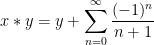
Exercise 22 Let
![\displaystyle \exp([X,Y]) = \lim_{n \rightarrow \infty} (\exp(X/n) \exp(Y/n)](https://s0.wp.com/latex.php?latex=%5Cdisplaystyle++%5Cexp%28%5BX%2CY%5D%29+%3D+%5Clim_%7Bn+%5Crightarrow+%5Cinfty%7D+%28%5Cexp%28X%2Fn%29+%5Cexp%28Y%2Fn%29+&bg=ffffff&fg=000000&s=0&c=20201002)


33 comments
Comments feed for this article
2 September, 2011 at 3:56 am
Combinatorics versus geometric… | chorasimilarity
[…] of using knowledge concerning topological groups in order to study discrete approximate groups, as Tao proposes in his new course, it is about discrete finitely generated groups with polynomial growth which, as Gromov taught us, […]
2 September, 2011 at 4:31 am
tanaka
Thank you for your good post.
By the way ,In Remark2, where does “Y” comes from?
[Oops, that was meant to be an X. Corrected, thanks – T.]
2 September, 2011 at 6:50 pm
254A, Notes 1: Lie groups, Lie algebras, and the Baker-Campbell-Hausdorff formula (via What's new) « Human Mathematics
[…] 254A, Notes 1: Lie groups, Lie algebras, and the Baker-Campbell-Hausdorff formula (via What's new) By human mathematics In this set of notes, we describe the basic analytic structure theory of Lie groups, by relating them to the simpler concept of a Lie algebra. Roughly speaking, the Lie algebra encodes the “infinitesimal” structure of a Lie group, but is a simpler object, being a vector space rather than a nonlinear manifold. Nevertheless, thanks to the fundamental theorems of Lie, the Lie algebra can be used to reconstruct the Lie group (at a local l … Read More […]
3 September, 2011 at 5:51 am
David Speyer
Typo: In the sentence beginning “However, we will use (iv)”, I imagine you mean (iii). [Corrected, thanks – T.]
5 September, 2011 at 2:45 pm
E. Mehmet Kiral
The fifth bullet point in exercise 6 seems to have a typo, $\mathbb{R}$ versus $\mathbb{C}$.
5 September, 2011 at 3:24 pm
Erik
It looks like you should have “..are well defined and lie in ” and
” and  instead of
  in example 1. [Corrected, thanks, although
  is actually not a typo. -T.]
7 September, 2011 at 5:01 am
Weekly Picks « Mathblogging.org — the Blog
[…] compactness theorem, n-Category Café on Hadwiger’s theorem, Terry Tao starting a series of posts on Hilbert’s fifth problem, and Vismath (in German, translation) and 0xDE on tilings. Also […]
8 September, 2011 at 2:10 pm
254A, Notes 2: Building Lie structure from representations and metrics « What’s new
[…] one-parameter subgroups to convert from the nonlinear setting to the linear setting. Recall from the previous notes that in a Lie group , the one-parameter subgroups are in one-to-one correspondence with the Lie […]
18 September, 2011 at 4:00 am
pavel zorin
Dear Prof. Tao,
I have some trouble with Exercise 9(v). Even in the easiest situation, that of Exercise 16(17), I keep getting terms like instead of |y-z| in the estimates. With the radial homogeneity assumption the two are equal, but otherwise there remains an error of O(|z|)². What can be done about it?
best regards,
pavel
18 September, 2011 at 9:23 am
Terence Tao
Ah yes, this requires an estimate which wasn’t explicitly in the previous exercises but which I’ve now added as Exercise 9(viii) (note that there has been some renumbering of exercises).
20 September, 2011 at 12:42 pm
pavel zorin
Thank you, this has helped me to show the Lipschitzianity of left and right translation, and thus Ex. 9 (vi) and (viii). I am however still lost with (vii), the asymptotics for .
.
What I think I can show is that it is up to an arbitrarily small relative error, if
  is small enough (from the analogous result
  up to a small relative error). Unfortunately, this is much weaker then the error being
  .
.
best regards,
pavel
20 September, 2011 at 1:47 pm
Terence Tao
Oops, that bound is indeed too strong to be true in general. I’ve replaced it with the bilipschitz bound as you indicated (which is what is actually needed going forward in the argument.)
31 March, 2013 at 3:28 am
THLee
I am looking for proofs for equivalence of any decomposition of a general anti-hermitain matrix when canonical coordinates of the first kind is mapped to the second kind in exponential map of SU(N) group. Can anyone suggest me any textbook or reference for this question?
20 September, 2011 at 5:18 pm
Erik
I’m having trouble understanding the term in exercise 10 (ii). I think this means the exponential map of a member of the equivalence class
  – in other words, a curve
  in
in  . But then this can’t be equal to the limit on the right since
  is (somewhat) arbitrary. Also, what does it mean to say that
  is sufficiently small.
20 September, 2011 at 6:25 pm
Terence Tao
Note that while there are multiple curves with the same derivative
  at zero, it will turn out that each of these curves ends up with the same limiting value of
  , thus the apparent ambiguity of
  will disappear in the limit.
In any event, in a local group, G is a subset of a Euclidean space, so one can use the Euclidean definition of
  in this case if one wishes.
20 September, 2011 at 7:28 pm
Erik
Thank you
27 September, 2011 at 3:29 pm
254A, Notes 3: Haar measure and the Peter-Weyl theorem « What’s new
[…] the last few notes, we have been steadily reducing the amount of regularity needed on a topological group in […]
8 October, 2011 at 11:11 am
Anonymous
Professor Tao,
In exercise 14, should G and H be local Lie groups?
[Corrected, thanks – T.]
8 October, 2011 at 9:53 pm
alingalatan
At the beginning of the proof of Proposition 9, shouldn’t it be , and not just $\rho_{\exp(tx)}^{left} x$?
[Corrected, thanks – T.]
28 October, 2011 at 1:35 am
Bruce Bartlett
I think that another way of integrating a Lie algebra to a Lie group (this is in regard to Remark 5), which doesn’t proceed via Ado’s theorem, is to define the group elements as equivalence classes of paths in the Lie algebra. My understanding is that there are two different equivalence relations one can put on the paths: the first can be found in the book “Lie Groups” by Duistermaat and Kolk, and the second can be found in Segal’s section of the book “Lectures on Lie Groups and Lie Algebras” by Carter, Segal and Macdonald. Both of these give rise to the same group I believe.
28 October, 2011 at 10:15 am
Terence Tao
I took a look at Carter-Segal-Macdonald (our library doesn’t have Duistermaat-Kolk). Unfortunately they omit the most crucial step of the argument, namely to show that two short paths are equivalent whenever they integrate out (via the infinitesimal form of BCH, i.e. Lemma 14 above) to the same element of the Lie algebra; they prove it using Ado’s theorem, but don’t indicate how to do it without that theorem (other than to say that it is “difficult”). So I suspect that the difficulty is simply being moved elsewhere.
29 October, 2011 at 11:25 am
Associativity of the Baker-Campbell-Hausdorff formula « What’s new
[…] for instance these notes of mine for a proof of this formula (it is for , but one easily obtains a similar proof for […]
5 March, 2012 at 10:43 pm
Johnny
I think ready solutions makes it easier.
I use Differential Geometry Library:
http://digi-area.com/DifferentialGeometryLibrary/
5 May, 2012 at 1:06 pm
alabair
I think there’s a typo in the definition 4 of the tangent space.
M instead of G.
7 October, 2012 at 6:56 pm
Some notes on Weyl quantisation « What’s new
[…] as well as exponential coordinates (of the first kind) on Lie groups, discussed for instance in this previous blog post. In contrast, the Kohn-Nirenberg quantisation […]
27 April, 2013 at 9:25 pm
Notes on the classification of complex Lie algebras | What's new
[…] counterparts in the category of Lie algebras (often with exactly the same terminology). See this previous blog post for more discussion about the connection between Lie algebras and Lie groups (that post was focused […]
5 September, 2013 at 9:23 pm
Notes on simple groups of Lie type | What's new
[…] (This statement can be made more precise using the Baker-Campbell-Hausdorff formula, discussed in this previous post.) On the other hand, every connected Lie group has a universal cover with the same Lie algebra […]
8 March, 2015 at 9:46 pm
Hao Zhuang
Reblogged this on Exponentials.
9 March, 2015 at 12:21 am
Anonymous
In definition 4, it seems that the (undefined) (appearing in line 4 and several other places) should be
  .
.
[Corrected, thanks – T.]
22 May, 2017 at 5:55 pm
Quantitative continuity estimates | What's new
[…] We remark that further manipulation of (iv) of the above exercise using the fundamental theorem of calculus eventually leads to the Baker-Campbell-Hausdorff-Dynkin formula, as discussed in this previous blog post. […]
20 April, 2019 at 12:28 pm
Arturo Rodríguez Fanlo
Dear Prof. Tao,
Thank you very much. If it is possible, I would sincerely appreciate any hint to show the lower bound of point (vii) of exercise 9:
In a local group, there is
  such that for any natural number
  and any
  with
with 
Again, thank you very much for everything.
Best wishes,
Arturo
20 April, 2019 at 3:15 pm
Terence Tao
Can you do the case ? You may find it helpful to write
  and try to estimate both
  and
and  in terms of
  .
.
29 April, 2019 at 10:27 am
Arturo Rodriguez Fanlo
Dear Prof. Tao,
Thank you very much for your attention.
Best wishes,
Arturo