Van Vu and I have just uploaded to the arXiv our paper A central limit theorem for the determinant of a Wigner matrix, submitted to Adv. Math.. It studies the asymptotic distribution of the determinant  of a random Wigner matrix (such as a matrix drawn from the Gaussian Unitary Ensemble (GUE) or Gaussian Orthogonal Ensemble (GOE)).
Before we get to these results, let us first discuss the simpler problem of studying the determinant  of a random iid matrix
  , such as a real gaussian matrix (where all entries are independently and identically distributed using the standard real normal distribution
  ), a complex gaussian matrix (where all entries are independently and identically distributed using the standard complex normal distribution
  , thus the real and imaginary parts are independent with law
  ), or the random sign matrix (in which all entries are independently and identically distributed according to the Bernoulli distribution
  (with a
  chance of either sign). More generally, one can consider a matrix
  in which all the entries
  are independently and identically distributed with mean zero and variance
  .
.
We can expand using the Leibniz expansion
where  ranges over the permutations of
  , and
, and  is the product

From the iid nature of the , we easily see that each has mean zero and variance one, and are pairwise uncorrelated as  varies. We conclude that has mean zero and variance
  (an observation first made by Turán). In particular, from Chebyshev’s inequality we see that is typically of size
  .
.
It turns out, though, that this is not quite best possible. This is easiest to explain in the real gaussian case, by performing a computation first made by Goodman. In this case, is clearly symmetrical, so we can focus attention on the magnitude  . We can interpret this quantity geometrically as the volume of an
  -dimensional parallelopiped whose generating vectors
  are independent real gaussian vectors in
  (i.e. their coefficients are iid with law
  ). Using the classical base-times-height formula, we thus have

where  is the
  -dimensional linear subspace of spanned by
  (note that , having an absolutely continuous joint distribution, are almost surely linearly independent). Taking logarithms, we conclude

Now, we take advantage of a fundamental symmetry property of the Gaussian vector distribution, namely its invariance with respect to the orthogonal group  . Because of this, we see that if we fix (and thus , the random variable
  has the same distribution as
  , or equivalently the
  distribution
where  are iid copies of . As this distribution does not depend on the , we conclude that the law of
  is given by the sum of independent -variables:

A standard computation shows that each  has mean
  and variance
  , and then a Taylor series (or Ito calculus) computation (using concentration of measure tools to control tails) shows that
  has mean
  and variance
  . As such, has mean
  and variance
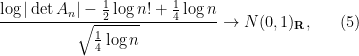
  . Applying a suitable version of the central limit theorem, one obtains the asymptotic law

where  denotes convergence in distribution. A bit more informally, we have

when is a real gaussian matrix; thus, for instance, the median value of is  . At first glance, this appears to conflict with the second moment bound
  of Turán mentioned earlier, but once one recalls that
  has a second moment of
  , we see that the two facts are in fact perfectly consistent; the upper tail of the normal distribution in the exponent in (4) ends up dominating the second moment.
It turns out that the central limit theorem (3) is valid for any real iid matrix with mean zero, variance one, and an exponential decay condition on the entries; this was first claimed by Girko, though the arguments in that paper appear to be incomplete. Another proof of this result, with more quantitative bounds on the convergence rate has been recently obtained by Hoi Nguyen and Van Vu. The basic idea in these arguments is to express the sum in (2) in terms of a martingale and apply the martingale central limit theorem.
If one works with complex gaussian random matrices instead of real gaussian random matrices, the above computations change slightly (one has to replace the real distribution with the complex distribution, in which the  are distributed according to the complex gaussian
  instead of the real one). At the end of the day, one ends up with the law
or more informally

(but note that this new asymptotic is still consistent with Turán’s second moment calculation).
We can now turn to the results of our paper. Here, we replace the iid matrices by Wigner matrices  , which are defined similarly but are constrained to be Hermitian (or real symmetric), thus
  for all
  . Model examples here include the Gaussian Unitary Ensemble (GUE), in which for
  and for
  , the Gaussian Orthogonal Ensemble (GOE), in which for and
  for , and the symmetric Bernoulli ensemble, in which for
  (with probability of either sign). In all cases, the upper triangular entries of the matrix are assumed to be jointly independent. For a more precise definition of the Wigner matrix ensembles we are considering, see the introduction to our paper.
The determinants of these matrices still have a Leibniz expansion. However, in the Wigner case, the mean and variance of the are slightly different, and what is worse, they are not all pairwise uncorrelated any more. For instance, the mean of is still usually zero, but equals  in the exceptional case when is a perfect matching (i.e. the union of exactly
 -cycles, a possibility that can of course only happen when is even). As such, the mean
  still vanishes when is odd, but for even it is equal to
(the fraction here simply being the number of perfect matchings on vertices). Using Stirling’s formula, one then computes that  is comparable to
  when is large and even. The second moment calculation is more complicated (and uses facts about the distribution of cycles in random permutations, mentioned in this previous post), but one can compute that
  is comparable to
  for GUE and
  for GOE. (The discrepancy here comes from the fact that in the GOE case, and
  can correlate when
  contains reversals of
  -cycles of for
  , but this does not happen in the GUE case.) For GUE, much more precise asymptotics for the moments of the determinant are known, starting from the work of Brezin and Hikami, though we do not need these more sophisticated computations here.
Our main results are then as follows.
Theorem 1 Let  be a Wigner matrix.
Thus, we informally have

when is drawn from GUE, or from another Wigner ensemble matching GUE to fourth order (and obeying some additional minor technical hypotheses); and

when is drawn from GOE, or from another Wigner ensemble matching GOE to fourth order. Again, these asymptotic limiting distributions are consistent with the asymptotic behaviour for the second moments.
The extension from the GUE or GOE case to more general Wigner ensembles is a fairly routine application of the four moment theorem for Wigner matrices, although for various technical reasons we do not quite use the existing four moment theorems in the literature, but adapt them to the log determinant. The main idea is to express the log-determinant as an integral

of the Stieltjes transform
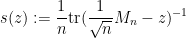
of . Strictly speaking, the integral in (7) is divergent at infinity (and also can be ill-behaved near zero), but this can be addressed by standard truncation and renormalisation arguments (combined with known facts about the least singular value of Wigner matrices), which we omit here. We then use a variant of the four moment theorem for the Stieltjes transform, as used by Erdos, Yau, and Yin (based on a previous four moment theorem for individual eigenvalues introduced by Van Vu and myself). The four moment theorem is proven by the now-standard Lindeberg exchange method, combined with the usual resolvent identities to control the behaviour of the resolvent (and hence the Stieltjes transform) with respect to modifying one or two entries, together with the delocalisation of eigenvector property (which in turn arises from local semicircle laws) to control the error terms.
Somewhat surprisingly (to us, at least), it turned out that it was the first part of the theorem (namely, the verification of the limiting law for the invariant ensembles GUE and GOE) that was more difficult than the extension to the Wigner case. Even in an ensemble as highly symmetric as GUE, the rows are no longer independent, and the formula (2) is basically useless for getting any non-trivial control on the log determinant. There is an explicit formula for the joint distribution of the eigenvalues of GUE (or GOE), which does eventually give the distribution of the cumulants of the log determinant, which then gives the required central limit theorem; but this is a lengthy computation, first performed by Delannay and Le Caer.
Following a suggestion of my colleague, Rowan Killip, we give an alternate proof of this central limit theorem in the GUE and GOE cases, by using a beautiful observation of Trotter, namely that the GUE or GOE ensemble can be conjugated into a tractable tridiagonal form. Let me state it just for GUE:
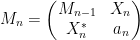
Proposition 2 (Tridiagonal form of GUE) Let  be the random tridiagonal real symmetric matrix
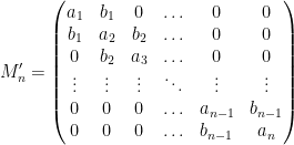
where the  are jointly independent real random variables, with
  being standard real Gaussians, and each
  having a -distribution:

where  are iid complex gaussians. Let be drawn from GUE. Then the joint eigenvalue distribution of is identical to the joint eigenvalue distribution of .
Proof: Let be drawn from GUE. We can write
where  is drawn from the
  GUE,
GUE, 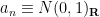 , and
, and  is a random gaussian vector with all entries iid with distribution . Furthermore,
  are jointly independent.
We now apply the tridiagonal matrix algorithm. Let  , then
  has the -distribution indicated in the proposition. We then conjugate by a unitary matrix
  that preserves the final basis vector
  , and maps
  to
to  . Then we have

where  is conjugate to . Now we make the crucial observation: because is distributed according to GUE (which is a unitarily invariant ensemble), and is a unitary matrix independent of , is also distributed according to GUE, and remains independent of both
  and
and  .
.
We continue this process, expanding  as
as
Applying a further unitary conjugation that fixes  but maps
  to
to  , we may replace by while transforming
  to another GUE matrix
  independent of
  . Iterating this process, we eventually obtain a coupling of to by unitary conjugations, and the claim follows.
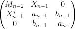
The determinant of a tridiagonal matrix is not quite as simple as the determinant of a triangular matrix (in which it is simply the product of the diagonal entries), but it is pretty close: the determinant  of the above matrix is given by solving the recursion

with  and
and  . Thus, instead of the product of a sequence of independent scalar distributions as in the gaussian matrix case, the determinant of GUE ends up being controlled by the product of a sequence of independent
  matrices whose entries are given by gaussians and distributions. In this case, one cannot immediately take logarithms and hope to get something for which the martingale central limit theorem can be applied, but some ad hoc manipulation of these
  matrix products eventually does make this strategy work. (Roughly speaking, one has to work with the logarithm of the Frobenius norm of the matrix first.)


13 comments
Comments feed for this article
28 November, 2011 at 10:47 pm
Greg Martin
Tiny typo, near the beginning when Chebyshev’s inequality is invoked: I think it should be $O(\sqrt{n!})$, with a factorial. [Corrected, thanks – T.]
29 November, 2011 at 2:22 am
Florent Benaych-Georges
Tiny typo : “Brezis” should be “Brezin”.
29 November, 2011 at 5:35 am
Peter Eichelsbacher
Tiny typos: in Theorem 3, Wigner matrix obeying Condition C1 (not C0),
and in the statement for the second moment: If M_n is drawn (twice). [Thanks, this will be corrected in the next revision of the ms – T.]
29 November, 2011 at 10:53 am
Xavier Gabaix
Tiny typo: right below (7), the definition of the Stieltjes transform has M in the numerator. [Corrected, thanks – T.]
29 November, 2011 at 2:40 pm
yunqing2010
Does the right hand of (7) miss a term like $$ \log | det (\frac{M_n}{\sqrt{n}} – \sqrt{-1}\infty) | $$ ?
29 November, 2011 at 3:01 pm
Terence Tao
Yes, one needs to truncate and renormalise the integral in order to eliminate the type divergence. This is discussed in detail in the paper, but I am omitting it in this post as it is a minor technical issue rather than a principal difficulty in the argument.
29 November, 2011 at 8:56 pm
Jayadev Athreya
In Theorem, 1, should it be M_n instead of A_n? [Corrected, thanks – T.]
1 December, 2011 at 12:04 pm
Craig
Tiny typo: Below (4), shouldn’t it be the median value of $$| det A_n |$$, not $$\log | det A_n |$$? [Corrected, thanks – T.]
1 December, 2011 at 3:11 pm
Anonymous
Tiny typos: “gaussian” –> “Gaussian” (A total of 12 time if my counting is correct; 13 including the tags.)
2 December, 2011 at 9:49 am
Antonio
i Professor Tarece Tao. I am a student of thirteen years and I love math and, therefore, gives great I would do the math. I wanted to ask whether Godel’s incompleteness theorems imply that in mathematics there are many problems unsolved? if it is true, then there are infinitely many complex problems as the ‘Riemann Hypothesis, or even more complex? Thanks Professor, thanks for all she is my idol, I wanted to also ask where can I buy your books? Sorry for my poor English because I’m Italian.
5 December, 2011 at 4:42 pm
kmkosinski
The conclusion from (2) is that , where
  are independent
  -variables. That is,
  and
and  are iid such that
  ,
, 
 distributed.
Hence, where
where  . That is,
  can be seen as a product of independent sums of iid random variables. Central limit theorem for such products (and its connection to Wishart determinants) has been discussed in G. Rempala, J. Wesolowski “Asymptotics for products of independent sums with an application to Wishart determinants”, Stat. Probab. Lett. 74 (2005) 129–138.
 with finite absolute moment of order
In particular, in this paper, it has been shown that for any sequence of iid positive square integrable random variables
tends in distribution to
Various other generalizations have been considered for asymptotics for products of (not necessarily independent) sums of random variables.
9 December, 2011 at 7:38 am
Anonymous
I am new to math research: what’s the significance of this? Should the references be included in the paper by professor Tao? Is the paper by prof. Tao completely derivative or not (is there an original contribution)?
11 June, 2012 at 9:29 pm
Random matrices: Universality of local spectral statistics of non-Hermitian matrices « What’s new
[…] paper), as well as central limit theorems for log-determinants of Wigner matrices (as we did in this other recent paper). In both of these papers, the main idea was to use the Four Moment Theorem for Wigner matrices […]