For each natural number  , let
, let  denote the quantity
where  denotes the
  prime. In other words, is the least quantity such that there are infinitely many intervals of length that contain
  or more primes. Thus, for instance, the twin prime conjecture is equivalent to the assertion that
  , and the prime tuples conjecture would imply that is equal to the diameter of the narrowest admissible tuple of cardinality (thus we conjecturally have ,
  ,
,  ,
,  ,
,  , and so forth; see this web page for further continuation of this sequence).
In 2004, Goldston, Pintz, and Yildirim established the bound  conditional on the Elliott-Halberstam conjecture, which remains unproven. However, no unconditional finiteness of
  was obtained (although they famously obtained the non-trivial bound
  ), and even on the Elliot-Halberstam conjecture no finiteness result on the higher was obtained either (although they were able to show
  on this conjecture). In the recent breakthrough of Zhang, the unconditional bound
  was obtained, by establishing a weak partial version of the Elliott-Halberstam conjecture; by refining these methods, the Polymath8 project (which I suppose we could retroactively call the Polymath8a project) then lowered this bound to
  .
.
With the very recent preprint of James Maynard, we have the following further substantial improvements:
Theorem 1 (Maynard’s theorem) Unconditionally, we have the following bounds:
-
 .
.
-
 for an absolute constant
  and any
  .
.
If one assumes the Elliott-Halberstam conjecture, we have the following improved bounds:
-
 .
.
-
 .
.
-
 for an absolute constant and any .
The final conclusion on Elliott-Halberstam is not explicitly stated in Maynard’s paper, but follows easily from his methods, as I will describe below the fold. (At around the same time as Maynard’s work, I had also begun a similar set of calculations concerning , but was only able to obtain the slightly weaker bound 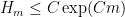 unconditionally.) In the converse direction, the prime tuples conjecture implies that should be comparable to
  . Granville has also obtained the slightly weaker explicit bound
  for any by a slight modification of Maynard’s argument.
The arguments of Maynard avoid using the difficult partial results on (weakened forms of) the Elliott-Halberstam conjecture that were established by Zhang and then refined by Polymath8; instead, the main input is the classical Bombieri-Vinogradov theorem, combined with a sieve that is closer in spirit to an older sieve of Goldston and Yildirim, than to the sieve used later by Goldston, Pintz, and Yildirim on which almost all subsequent work is based.
The aim of the Polymath8b project is to obtain improved bounds on  , and higher values of , either conditional on the Elliott-Halberstam conjecture or unconditional. The likeliest routes for doing this are by optimising Maynard’s arguments and/or combining them with some of the results from the Polymath8a project. This post is intended to be the first research thread for that purpose. To start the ball rolling, I am going to give below a presentation of Maynard’s results, with some minor technical differences (most significantly, I am using the Goldston-Pintz-Yildirim variant of the Selberg sieve, rather than the traditional “elementary Selberg sieve” that is used by Maynard (and also in the Polymath8 project), although it seems that the numerology obtained by both sieves is essentially the same). An alternate exposition of Maynard’s work has just been completed also by Andrew Granville.
— 1. Overview of argument —
Define an admissible  -tuple to be an increasing tuple
  of integers, which avoids at least one residue class modulo
  for each . For
  , let
, let ![{DHL[k_0,j_0]}](https://s0.wp.com/latex.php?latex=%7BDHL%5Bk_0%2Cj_0%5D%7D&bg=ffffff&fg=000000&s=0&c=20201002) denote the following claim:
denote the following claim:
Conjecture 2 () If  is an admissible -tuple, then there are infinitely many translates
  of that contain at least
  primes.
The prime tuples conjecture is then the assertion that holds for all  . Clearly, if
 ![{DHL[k_0,m+1]}](https://s0.wp.com/latex.php?latex=%7BDHL%5Bk_0%2Cm%2B1%5D%7D&bg=ffffff&fg=000000&s=0&c=20201002) is true, then we have
is true, then we have  whenever
  is an admissible -tuple. Theorem 1 then follows from the following claim:
Theorem 3 (Maynard’s theorem, DHL version) Unconditionally, we have the following bounds:
-
![{DHL[105,2]}](https://s0.wp.com/latex.php?latex=%7BDHL%5B105%2C2%5D%7D&bg=ffffff&fg=000000&s=0&c=20201002) .
.
- whenever is sufficiently large and
 .
.
If one assumes the Elliott-Halberstam conjecture, we have the following improved bounds:
-
![{DHL[5,2]}](https://s0.wp.com/latex.php?latex=%7BDHL%5B5%2C2%5D%7D&bg=ffffff&fg=000000&s=0&c=20201002) .
.
-
![{DHL[105,3]}](https://s0.wp.com/latex.php?latex=%7BDHL%5B105%2C3%5D%7D&bg=ffffff&fg=000000&s=0&c=20201002) .
.
- whenever is sufficiently large and
 .
.
Indeed, the  results then follow from using the admissible
  -tuple
  and the admissible
  -tuple


found by Engelsma (and recorded on this site). For the larger results, note that the bound is obeyed if  for a sufficiently large and is large enough, and the claim follows by using the observation that one can create an admissible -tuple of length
  by using the first primes past ; similarly if one assumes the Elliott-Halberstam conjecture. (Note as the are clearly non-decreasing in , it suffices to work with sufficiently large to obtain bounds such as .)
As in previous work, the conclusions are obtained by constructing a sieve weight with good properties. We use the same asymptotic notation as in the Polymath8a project, thus all quantities depend on an asymptotic parameter  unless explicitly declared to be fixed, and asymptotic notation such
  ,
,  or
or  is relative to this parameter. We let

and  as before. We let
  be the quantity
  when
when  is prime, and zero otherwise.
Lemma 4 (Criterion for  ) Let
) Let  and be fixed integers. Suppose that for each fixed admissible -tuple and each congruence class
  such that
  is coprime to
  for all
  , one can find a non-negative weight function
  , fixed quantities
  , a quantity
  , and a quantity
  such that one has the upper bound

the lower bound
for all  , and the key inequality

Then holds.
The  case of this lemma is Lemma 4.1 of the polymath8a paper. The general case is proven by an essentially identical argument, namely one considers the expression
uses the hypotheses (1), (2), (3) to show that this is positive for sufficiently large , and observing that the summand is only positive when  contain at least primes.
We recall the statement of the Elliott-Halberstam conjecture, for a given choice of parameter  :
:
If  and
and  is fixed, then
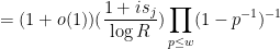
![\displaystyle \sum_{q \leq Q} \sup_{a \in ({\bf Z}/q{\bf Z})^\times} |\Delta(\Lambda 1_{[x,2x]}; a\ (q))| \ll x \log^{-A} x \ \ \ \ \ (4)](https://s0.wp.com/latex.php?latex=%5Cdisplaystyle++%5Csum_%7Bq+%5Cleq+Q%7D+%5Csup_%7Ba+%5Cin+%28%7B%5Cbf+Z%7D%2Fq%7B%5Cbf+Z%7D%29%5E%5Ctimes%7D+%7C%5CDelta%28%5CLambda+1_%7B%5Bx%2C2x%5D%7D%3B+a%5C+%28q%29%29%7C+%5Cll+x+%5Clog%5E%7B-A%7D+x+%5C+%5C+%5C+%5C+%5C+%284%29&bg=ffffff&fg=000000&s=0&c=20201002)
where

The Bombieri-Vinogradov theorem asserts that ![{EH[\theta]}](https://s0.wp.com/latex.php?latex=%7BEH%5B%5Ctheta%5D%7D&bg=ffffff&fg=000000&s=0&c=20201002) holds for all
holds for all  , while the Elliott-Halberstam conjecture asserts that holds for all .
In Polymath8a, the sieve weight  was constructed in terms of a smooth compactly supported one-variable function
  . A key innovation in Maynard’s work is to replace the sieve with one constructed using a smooth compactly supported multi-variable function
  , which affords significantly greater flexibility. More precisely, we will show
Proposition 5 (Sieve asymptotics) Suppose that holds for some fixed , and set  for some fixed
  . Let is a fixed symmetric smooth function supported on the simplex

Then one can find obeying the bounds (1), (2) with


where we use the shorthand

for the mixed partial derivatives of  .
.
(In fact, one can obtain asymptotics for (1), (2), rather than upper and lower bounds.)
(One can work with non-symmetric functions , but this does not improve the numerology; see the remark after (7.1) of Maynard’s paper.)
We prove this proposition in Section 2. We remark that if one restricts attention to functions of the form

for smooth and supported on ![{[0,1]}](https://s0.wp.com/latex.php?latex=%7B%5B0%2C1%5D%7D&bg=ffffff&fg=000000&s=0&c=20201002) , then
, then

and

and this claim was already essentially established back in this Polymath8a post (or see Proposition 4.1 and Lemma 4.7 of the Polymath8a paper for essentially these bounds). In that previous post (and also in the paper of Farkas, Pintz, and Revesz), the ratio  was optimised in this one-dimensional context using Bessel functions, and the method was unable to reach without an improvement to Bombieri-Vinogradov, or to reach
  even on Elliott-Halberstam. However, the additional flexibility afforded by the use of multi-dimensional cutoffs allows one to do better.
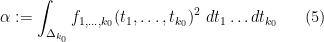
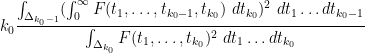
Combining Proposition 5 with Lemma 4, we obtain the following conclusion. For each , let  be the quantity

where ranges over all smooth symmetric functions that are supported on the simplex  . Equivalently, by substituting
  and using the fundamental theorem of calculus, followed by an approximation argument to remove the smoothness hypotheses on
  , we have

where ranges over all bounded measurable functions supported on . Then we have
Corollary 6 Let  be such that holds, and let , be integers such that

Then holds.
To use this corollary, we simply have to locate test functions that give as large a lower bound for as one can manage; this is a purely analytic problem that no longer requires any further number-theoretic input.
In particular, Theorem 3 follows from the following lower bounds:
Proposition 7
The first two cases of this proposition are obtained numerically (see Section 7 of Maynard’s paper), by working with functions that of the special form

for various real coefficients  and non-negative integers
  , where

and

In Maynard’s paper, the ratio
in this case is computed to be

where  is the
  matrix with entries
  ,
,  is the
  matrix with
  entry equal to

where

and  is the matrix with entry equal to

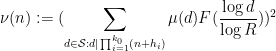
where  is the quantity

One then optimises the ratio  by linear programming methods (a similar idea appears in the original paper of Goldston, Pintz, and Yildirim) to obtain a lower bound for for
  and
and  .
.
The final case is established in a different manner; we give a proof of the slightly weaker bound

in Section 3.
— 2. Sieve asymptotics —
We now prove Proposition 5. We use a Fourier-analytic method, similar to that in this previous blog post.
The sieve we will use is of the form


where  denotes the square-free integers and
  is the Möbius function This should be compared with the sieve
used in the previous blog post, which basically corresponds to the special case  .
.
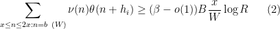
We begin with (1). Using (10), we may rearrange the left-hand side of (1) as


![\displaystyle \sum_{x \leq n \leq 2x: n = b\ (W); [d_j,d'_j] | n+h_j \hbox{ for all } j=1,\ldots,k_0} 1.](https://s0.wp.com/latex.php?latex=%5Cdisplaystyle++%5Csum_%7Bx+%5Cleq+n+%5Cleq+2x%3A+n+%3D+b%5C+%28W%29%3B+%5Bd_j%2Cd%27_j%5D+%7C+n%2Bh_j+%5Chbox%7B+for+all+%7D+j%3D1%2C%5Cldots%2Ck_0%7D+1.&bg=ffffff&fg=000000&s=0&c=20201002)
Observe that as the numbers have no common factor when  , the inner sum vanishes unless the quantities
 ![{[d_1,d'_1],\ldots,[d_{k_0},d'_{k_0}]}](https://s0.wp.com/latex.php?latex=%7B%5Bd_1%2Cd%27_1%5D%2C%5Cldots%2C%5Bd_%7Bk_0%7D%2Cd%27_%7Bk_0%7D%5D%7D&bg=ffffff&fg=000000&s=0&c=20201002) are coprime, in which case this inner sum can be estimated as
are coprime, in which case this inner sum can be estimated as
![\displaystyle \frac{x}{W [d_1,d'_1] \ldots [d_{k_0},d'_{k_0}]}+O(1).](https://s0.wp.com/latex.php?latex=%5Cdisplaystyle++%5Cfrac%7Bx%7D%7BW+%5Bd_1%2Cd%27_1%5D+%5Cldots+%5Bd_%7Bk_0%7D%2Cd%27_%7Bk_0%7D%5D%7D%2BO%281%29.&bg=ffffff&fg=000000&s=0&c=20201002)
Also, at least one of the two products involving will vanish unless one has

Let us first deal with the contribution of the error term  to (1). This contribution may be bounded by

which sums to 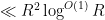 ; since and
  , we conclude that this contribution is negligible.
To conclude the proof of (1), it thus suffices to show that
![\displaystyle \sum_{d_1,\ldots,d_{k_0},d'_1,\ldots,d'_{k_0}\in {\cal S}: [d_1,d'_1],\ldots,[d_{k_0},d'_{k_0}] \hbox{ coprime}} (\prod_{j=1}^{k_0} \mu(d_j) \mu(d'_j)) \ \ \ \ \ (11)](https://s0.wp.com/latex.php?latex=%5Cdisplaystyle++%5Csum_%7Bd_1%2C%5Cldots%2Cd_%7Bk_0%7D%2Cd%27_1%2C%5Cldots%2Cd%27_%7Bk_0%7D%5Cin+%7B%5Ccal+S%7D%3A+%5Bd_1%2Cd%27_1%5D%2C%5Cldots%2C%5Bd_%7Bk_0%7D%2Cd%27_%7Bk_0%7D%5D+%5Chbox%7B+coprime%7D%7D+%28%5Cprod_%7Bj%3D1%7D%5E%7Bk_0%7D+%5Cmu%28d_j%29+%5Cmu%28d%27_j%29%29+%5C+%5C+%5C+%5C+%5C+%2811%29&bg=ffffff&fg=000000&s=0&c=20201002)
![\displaystyle \frac{f( \frac{\log d_1}{\log R}, \ldots, \frac{\log d_{k_0} }{\log R} ) f( \frac{\log d'_1}{\log R}, \ldots, \frac{\log d'_{k_0} }{\log R} )}{[d_1,d'_1] \ldots [d_k,d'_k]}](https://s0.wp.com/latex.php?latex=%5Cdisplaystyle++%5Cfrac%7Bf%28+%5Cfrac%7B%5Clog+d_1%7D%7B%5Clog+R%7D%2C+%5Cldots%2C+%5Cfrac%7B%5Clog+d_%7Bk_0%7D+%7D%7B%5Clog+R%7D+%29+f%28+%5Cfrac%7B%5Clog+d%27_1%7D%7B%5Clog+R%7D%2C+%5Cldots%2C+%5Cfrac%7B%5Clog+d%27_%7Bk_0%7D+%7D%7B%5Clog+R%7D+%29%7D%7B%5Bd_1%2Cd%27_1%5D+%5Cldots+%5Bd_k%2Cd%27_k%5D%7D+&bg=ffffff&fg=000000&s=0&c=20201002)
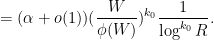
Next, we smoothly extend the function to a smooth compactly supported function  , which by abuse of notation we will continue to refer to as . By Fourier inversion, we may then express in the form
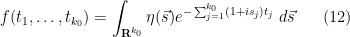
where 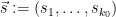 and where
  is a smooth function obeying the rapid decay bounds

for any fixed  . The left-hand side of (11) may then be rewritten as
where  and
and
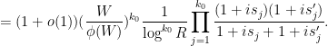
![\displaystyle H(\vec s, \vec s') := \sum_{d_1,\ldots,d_{k_0},d'_1,\ldots,d'_{k_0}\in {\cal S}: [d_1,d'_1],\ldots,[d_{k_0},d'_{k_0}] \hbox{ coprime}} (\prod_{j=1}^{k_0} \mu(d_j) \mu(d'_j))](https://s0.wp.com/latex.php?latex=%5Cdisplaystyle++H%28%5Cvec+s%2C+%5Cvec+s%27%29+%3A%3D+%5Csum_%7Bd_1%2C%5Cldots%2Cd_%7Bk_0%7D%2Cd%27_1%2C%5Cldots%2Cd%27_%7Bk_0%7D%5Cin+%7B%5Ccal+S%7D%3A+%5Bd_1%2Cd%27_1%5D%2C%5Cldots%2C%5Bd_%7Bk_0%7D%2Cd%27_%7Bk_0%7D%5D+%5Chbox%7B+coprime%7D%7D+%28%5Cprod_%7Bj%3D1%7D%5E%7Bk_0%7D+%5Cmu%28d_j%29+%5Cmu%28d%27_j%29%29+&bg=ffffff&fg=000000&s=0&c=20201002)
![\displaystyle \frac{\prod_{j=1}^{k_0} d_j^{-(1+is_j)/\log R} (d'_j)^{-(1+is'_j)/\log R}}{[d_1,d'_1] \ldots [d_k,d'_k]}.](https://s0.wp.com/latex.php?latex=%5Cdisplaystyle++%5Cfrac%7B%5Cprod_%7Bj%3D1%7D%5E%7Bk_0%7D+d_j%5E%7B-%281%2Bis_j%29%2F%5Clog+R%7D+%28d%27_j%29%5E%7B-%281%2Bis%27_j%29%2F%5Clog+R%7D%7D%7B%5Bd_1%2Cd%27_1%5D+%5Cldots+%5Bd_k%2Cd%27_k%5D%7D.+&bg=ffffff&fg=000000&s=0&c=20201002)
We may factorise  as an Euler product


In particular, we have the crude bound

combining this with (13) we see that the contribution to (14) in which  or
or  is negligible, so we may restrict the integral in (14) to the region
  . In this region, we have the Euler product approximations


where we have used the bound  and the asymptotic
  for
for  . Since also
  , we conclude that

Using (13) again to dispose of the  error term, and then using (13) once more to remove the restriction to , we thus reduce to verifying the identity

But from repeatedly differentiating (12) under the integral sign, one has

and thus

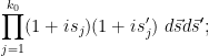
integrating this for  using Fubini’s theorem (and (13)), the claim then follows from (5). This concludes the proof of (1).
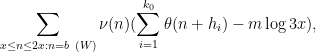
Now we prove (2). We will just prove the claim for  , as the other cases follow similarly using the symmetry hypothesis on . The left-hand side of (2) may then be expanded as


![\displaystyle \sum_{x \leq n \leq 2x: n = b\ (W); [d_j,d'_j] | n+h_j \hbox{ for all } j=1,\ldots,k_0} \theta(n+h_{k_0}).](https://s0.wp.com/latex.php?latex=%5Cdisplaystyle++%5Csum_%7Bx+%5Cleq+n+%5Cleq+2x%3A+n+%3D+b%5C+%28W%29%3B+%5Bd_j%2Cd%27_j%5D+%7C+n%2Bh_j+%5Chbox%7B+for+all+%7D+j%3D1%2C%5Cldots%2Ck_0%7D+%5Ctheta%28n%2Bh_%7Bk_0%7D%29.+&bg=ffffff&fg=000000&s=0&c=20201002)
Observe that the summand vanishes unless  (note that
  is comparable to and thus exceeds
  ). So we may simplify the above expression to

![\displaystyle \sum_{x \leq n \leq 2x: n = b\ (W); [d_j,d'_j] | n+h_j \hbox{ for all } j=1,\ldots,k_0-1} \theta(n+h_{k_0}).](https://s0.wp.com/latex.php?latex=%5Cdisplaystyle++%5Csum_%7Bx+%5Cleq+n+%5Cleq+2x%3A+n+%3D+b%5C+%28W%29%3B+%5Bd_j%2Cd%27_j%5D+%7C+n%2Bh_j+%5Chbox%7B+for+all+%7D+j%3D1%2C%5Cldots%2Ck_0-1%7D+%5Ctheta%28n%2Bh_%7Bk_0%7D%29.+&bg=ffffff&fg=000000&s=0&c=20201002)
As in the estimation of (1), the summand vanishes unless ![{[d_1,d'_1],\ldots,[d_{k_0-1},d'_{k_0-1}]}](https://s0.wp.com/latex.php?latex=%7B%5Bd_1%2Cd%27_1%5D%2C%5Cldots%2C%5Bd_%7Bk_0-1%7D%2Cd%27_%7Bk_0-1%7D%5D%7D&bg=ffffff&fg=000000&s=0&c=20201002) are coprime, and if
are coprime, and if

Let  obey the above constraints. For any modulus
  , define the discrepancy

Since and is fixed, the hypothesis implies that

for any fixed . On the other hand, the sum
![\displaystyle \sum_{x \leq n \leq 2x: n = b\ (W); [d_j,d'_j] | n+h_j \hbox{ for all } j=1,\ldots,k_0-1} \theta(n+h_{k_0})](https://s0.wp.com/latex.php?latex=%5Cdisplaystyle+%5Csum_%7Bx+%5Cleq+n+%5Cleq+2x%3A+n+%3D+b%5C+%28W%29%3B+%5Bd_j%2Cd%27_j%5D+%7C+n%2Bh_j+%5Chbox%7B+for+all+%7D+j%3D1%2C%5Cldots%2Ck_0-1%7D+%5Ctheta%28n%2Bh_%7Bk_0%7D%29&bg=ffffff&fg=000000&s=0&c=20201002)
can, by the Chinese remainder theorem, be rewritten in the form

where
![\displaystyle q := W \prod_{j=0}^{k_0-1} [d_j,d'_j] \ \ \ \ \ (17)](https://s0.wp.com/latex.php?latex=%5Cdisplaystyle++q+%3A%3D+W+%5Cprod_%7Bj%3D0%7D%5E%7Bk_0-1%7D+%5Bd_j%2Cd%27_j%5D+%5C+%5C+%5C+%5C+%5C+%2817%29&bg=ffffff&fg=000000&s=0&c=20201002)
and  is a primitive residue class; note that does not exceed
  . By (15), this expression can then be written as
![\displaystyle \frac{x}{\phi(W) \prod_{j=0}^{k_0-1} \phi([d_j,d'_j])} + O( E(W \prod_{j=0}^{k_0-1} [d_j,d'_j]) ).](https://s0.wp.com/latex.php?latex=%5Cdisplaystyle++%5Cfrac%7Bx%7D%7B%5Cphi%28W%29+%5Cprod_%7Bj%3D0%7D%5E%7Bk_0-1%7D+%5Cphi%28%5Bd_j%2Cd%27_j%5D%29%7D+%2B+O%28+E%28W+%5Cprod_%7Bj%3D0%7D%5E%7Bk_0-1%7D+%5Bd_j%2Cd%27_j%5D%29+%29.&bg=ffffff&fg=000000&s=0&c=20201002)
Let us first control the error term, which may be bounded by
![\displaystyle O( \sum_{d_1,\ldots,d_{k_0-1},d'_1,\ldots,d'_{k_0-1}: d_1 \ldots d_{k_0-1}, d'_1 \ldots d'_{k_0-1} \leq R} E(W \prod_{j=0}^{k_0-1} [d_j,d'_j]) ).](https://s0.wp.com/latex.php?latex=%5Cdisplaystyle++O%28+%5Csum_%7Bd_1%2C%5Cldots%2Cd_%7Bk_0-1%7D%2Cd%27_1%2C%5Cldots%2Cd%27_%7Bk_0-1%7D%3A+d_1+%5Cldots+d_%7Bk_0-1%7D%2C+d%27_1+%5Cldots+d%27_%7Bk_0-1%7D+%5Cleq+R%7D+E%28W+%5Cprod_%7Bj%3D0%7D%5E%7Bk_0-1%7D+%5Bd_j%2Cd%27_j%5D%29+%29.&bg=ffffff&fg=000000&s=0&c=20201002)
Note that for any  , there are
  choices of
  for which (17) holds. Thus we may bound the previous expression by

By the Cauchy-Schwarz inequality and (16), this expression may be bounded by

for any fixed  . On the other hand, we have the crude bound
  , as well as the standard estimate
(see e.g. Corollary 2.15 of Montgomery-Vaughan). Putting all this together, we conclude that the contribution of the error term to (2) is negligible. To conclude the proof of (2), it thus suffices to show that
![\displaystyle \frac{f( \frac{\log d_1}{\log R}, \ldots, \frac{\log d_{k_0-1} }{\log R}, 0 ) f( \frac{\log d'_1}{\log R}, \ldots, \frac{\log d'_{k_0-1} }{\log R}, 0 )}{\prod_{j=0}^{k_0-1} \phi([d_j,d'_j])}](https://s0.wp.com/latex.php?latex=%5Cdisplaystyle++%5Cfrac%7Bf%28+%5Cfrac%7B%5Clog+d_1%7D%7B%5Clog+R%7D%2C+%5Cldots%2C+%5Cfrac%7B%5Clog+d_%7Bk_0-1%7D+%7D%7B%5Clog+R%7D%2C+0+%29+f%28+%5Cfrac%7B%5Clog+d%27_1%7D%7B%5Clog+R%7D%2C+%5Cldots%2C+%5Cfrac%7B%5Clog+d%27_%7Bk_0-1%7D+%7D%7B%5Clog+R%7D%2C+0+%29%7D%7B%5Cprod_%7Bj%3D0%7D%5E%7Bk_0-1%7D+%5Cphi%28%5Bd_j%2Cd%27_j%5D%29%7D+&bg=ffffff&fg=000000&s=0&c=20201002)
But this can be proven by repeating the arguments used to prove (11) (with replaced by  , and
, and  replaced by
  ); the presence of the Euler totient function causes some factors of
  in that analysis to be replaced by
  , but this turns out to have a negligible impact on the final asymptotics since
  . This concludes the proof of (2) and hence Proposition 5.
Remark 1 An inspection of the above arguments shows that the simplex can be enlarged slightly to the region

however this only leads to a tiny improvement in the numerology. It is interesting to note however that in the  case,
case,  is the unit square
 ![{[0,1]^2}](https://s0.wp.com/latex.php?latex=%7B%5B0%2C1%5D%5E2%7D&bg=ffffff&fg=000000&s=0&c=20201002) , and by taking
, and by taking  and taking
  close to
  , one can come “within an epsilon” of establishing
 ![{DHL[2,2]}](https://s0.wp.com/latex.php?latex=%7BDHL%5B2%2C2%5D%7D&bg=ffffff&fg=000000&s=0&c=20201002) (and in particular, the twin prime conjecture) from the full Elliott-Halberstam conjecture; this fact was already essentially observed by Bombieri, using the weight
(and in particular, the twin prime conjecture) from the full Elliott-Halberstam conjecture; this fact was already essentially observed by Bombieri, using the weight  rather than the Selberg sieve. (Strictly speaking, to establish (1) in this context, one needs the Elliott-Halberstam conjecture not only for
  , but also for other arithmetic functions with a suitable Dirichlet convolution
  structure; we omit the details.)
Remark 2 It appears that the ![{MPZ[\varpi,\delta]}](https://s0.wp.com/latex.php?latex=%7BMPZ%5B%5Cvarpi%2C%5Cdelta%5D%7D&bg=ffffff&fg=000000&s=0&c=20201002) conjecture studied in Polymath8a can serve as a substitute for
conjecture studied in Polymath8a can serve as a substitute for ![{EH[\frac{1}{2}+2\varpi]}](https://s0.wp.com/latex.php?latex=%7BEH%5B%5Cfrac%7B1%7D%7B2%7D%2B2%5Cvarpi%5D%7D&bg=ffffff&fg=000000&s=0&c=20201002) in Corollary 6, except that one also has to impose an additional constraint on the function (or ), namely that it is supported in the cube
in Corollary 6, except that one also has to impose an additional constraint on the function (or ), namely that it is supported in the cube ![{[0, \frac{\delta}{1/4 +\varpi}]^{k_0}}](https://s0.wp.com/latex.php?latex=%7B%5B0%2C+%5Cfrac%7B%5Cdelta%7D%7B1%2F4+%2B%5Cvarpi%7D%5D%5E%7Bk_0%7D%7D&bg=ffffff&fg=000000&s=0&c=20201002) (in order to keep the moduli involved appropriately smooth). Perhaps as a first approximation, we should ignore the role of
(in order to keep the moduli involved appropriately smooth). Perhaps as a first approximation, we should ignore the role of  , and just pretend that is as good as . In particular, inserting our most optimistic value of
  obtained by Polymath8, namely
  , we can in principle take
  as large as
  , although this only is a
  improvement or so over the Bombieri-Vinogradov inequality.
— 3. Large computations —
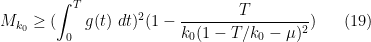
We now give a proof of (9) for sufficiently large . We use the ansatz

where  is the tensor product

and  is supported on some interval
 ![{[0,T]}](https://s0.wp.com/latex.php?latex=%7B%5B0%2CT%5D%7D&bg=ffffff&fg=000000&s=0&c=20201002) and normalised so that
and normalised so that

The function is clearly symmetric and supported on . We now estimate the numerator and denominator of the ratio
that lower bounds .
For the denominator, we bound by and use Fubini’s theorem and (8) to obtain the upper bound

and thus
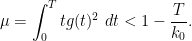
Now we observe that

whenever  , and so we have the lower bound

We interpret this probabilistically. Let  be independent, identically distributed non-negative real random variables with probability density
  ; this is well-defined thanks to (18). Observe that
  is the joint probability density of
  , and so

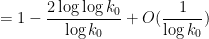
We will lower bound this probability using the Chebyshev inequality. (In my own calculations, I had used the Hoeffding inequality instead, but it seems to only give a slightly better bound in the end for (perhaps saving one or two powers of ).) In order to exploit the law of large numbers, we would like the mean  of
of  , where
  , to be less than
  :
:

The variance of is times the variance of a single  , which we can bound (somewhat crudely) by

Thus by Chebyshev’s inequality, we have

To clean things up a bit we bound by to obtain the simpler bound

assuming now that  . In particular,
  , so we have the cleaner bound

To summarise, we have shown that
whenever ![{g: [0,T] \rightarrow {\bf R}}](https://s0.wp.com/latex.php?latex=%7Bg%3A+%5B0%2CT%5D+%5Crightarrow+%7B%5Cbf+R%7D%7D&bg=ffffff&fg=000000&s=0&c=20201002) is such that
is such that

and
One can optimise this carefully to give (8) (as is done in Maynard’s paper), but for the purposes of establishing the slightly weaker bound (9), we can use  of the form

with  and
and  . With the normalisation (20) we have

so

and

and thus

while
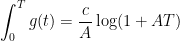

which gives the claim.

.
.


161 comments
Comments feed for this article
19 November, 2013 at 11:04 pm
Terence Tao
There are a couple of initial directions to proceed from here, I think. One is to get better bounds on ; as pointed out by Eytan in the previous thread; Maynard is working with functions of the first two symmetric polynomials
  and
and  , but in principle all the symmetric functions are available. (Though perhaps before doing that we should at least get to the point where we can replicate Maynard’s computations; note that he has supplied a Mathematica notebook in the source code of his arXiv file, although it is slightly nontrivial to extract it from the arXiv interface.) Another is to use MPZ instead of Bombieri-Vinogradov, but this puts an additional constraint on the test function F that has to be accounted for, and is likely to have a modest impact on
  (improving this quantity by about 5% or so). A third thing to do is to try to enlarge the allowable support of the function F, as per Remark 1; this is likely to be a very modest gain (basically it should shift
  downward by 1 or so), but this could be significant for bounding
  on EH, as it may shift
  down from 5 to 4 (bringing the
  bound from 12 to 8).
Indeed, it seems that focusing on the case (assuming EH) may well be the best place to start, as the numerics should be fast and one can work a certain number of things out by hand in such low-dimensional cases.
20 November, 2013 at 3:51 am
Andrew Sutherland
With Maynard’s permission, I have posted a copy of his Mathematica notebook source as a text file here.
20 November, 2013 at 6:19 am
Anonymous
Any chance I can make you (on anyone else) convert the text document into a notebook? I’m totally new to Mathematica and would like to play around with a fully working notebook. (I’m using v9.0 in case it is important.) [Sorry for interrupting the thread.]
20 November, 2013 at 7:51 am
Andrew Sutherland
You should be able to just save the file with the extension .nb and mathematica will be happy to load it as a notebook.
20 November, 2013 at 8:09 am
Anonymous
Thank you, Andrew.
@Terry: Just remove this post and my previous question if you want.
20 November, 2013 at 10:16 am
James Maynard
I don’t think you can get to (under EH) using just Remark 1 and higher symmetric polynomials (this seems to get only about half way numerically). That said, there are various possible small modifications (such as those you mention below) which might give enough of an improvement.
20 November, 2013 at 11:36 am
Vít Tuček
Did you try nonpolynomial symmetric functions? There is some work done on symmetric orthogonal polynomials on the standard simplex. See e.g. the section 3.3 of https://www.sciencedirect.com/science/article/pii/S0021904504002199 and https://www.sciencedirect.com/science/article/pii/S0377042700005045
20 November, 2013 at 1:03 pm
Eytan Paldi
A related idea is to use the transformation to have the weight function over the unit ball (which is perhaps simpler than the simplex).
20 November, 2013 at 3:16 pm
Vít Tuček
That’s precisely what is happening in the articles I’ve linked. The author then “constructs” some invariant orthogonal polynomials on the standard simplex. The problem is to find the matrix of with respect to the basis of orthogonal symmetric polynomials.
Of course, we can always take arbitrary polynomials in elementary symmetric functions (which give us all invariant polynomials) and evaluate the integrals numerically.
20 November, 2013 at 3:24 pm
James Maynard
I only looked very briefly at the numerical optimization with non-polynomial functions.
We know (Weierstrass) that polynomial approximations will converge to the optimal function. Moreover, I found that the numerical bounds from polynomial approximations seemed to converge quickly.
For , it is easy to use approximations involving higher symmetric polynomials, but there is only a very limited numerical improvement after having taken a low-degree approximation.
For things are more complicated, and convergence is a bit slower, so if there is some nicer basis of symmetric functions maybe thats worth looking at. That said, I would have guessed that it is computationally feasible to include higher degree symmetric polynomials and get a bound that is accurate enough to get the globally best value of
  (if we’re only following the method in my paper – with new ideas, such as MPZ this might no longer be true).
20 November, 2013 at 3:42 pm
Eytan Paldi
There is no need for numerical evaluation since any monomial in over the simplex is transformed to a monomial in
  over the unit ball whose integral is separable (by using spherical coordinates) with explicit expression in terms of beta functions (in this case factorials.)
19 November, 2013 at 11:14 pm
Polymath 8 – a Success! | Combinatorics and more
[…] Tao launched a followup polymath8b to improve the bounds for gaps between primes based on Maynard’s […]
19 November, 2013 at 11:21 pm
Gil Kalai
Naive questions: 1) Do the small gaps results apply to primes in arithmetic progressions? 2) Could there be a way to bootstrap results for k-tuples of prime in small intervals to get back results on 2-tuples. (The k-tuples result feels in some sense also stronger than the twin prime conjecture.)
20 November, 2013 at 8:03 am
Terence Tao
For (1), this should be possible. The original Goldston-Pintz-Yildirim results were extended to arithmetic progressions by Freiberg (http://arxiv.org/abs/1110.6624) and to more general sets of Bohr type by my student Benatar (http://arxiv.org/abs/1305.0348). In Maynard’s paper, it is noted that for the purposes of getting finite values for , the set of primes can be replaced by any other set that obeys a Bombieri-Vinogradov type theorem (at any level of distribution, not necessarily as large as 1/2), which includes the primes in arithmetic progressions (and also primes in fairly short intervals).
There may be some interplay between the k-tuple results and the 2-tuple results, but note that the set of primes we can detect in a k-tuple is rather sparse, we only catch about primes in such a tuple. Basically, Maynard’s construction gives, for each
  and each admissible tuple
  , a sieve weight
  (which is basically concentrated on a set in
 ![[x,2x]](https://s0.wp.com/latex.php?latex=%5Bx%2C2x%5D&bg=ffffff&fg=545454&s=0&c=20201002) of density about
of density about  ) with the property that if
 ![n \in [x,2x]](https://s0.wp.com/latex.php?latex=n+%5Cin+%5Bx%2C2x%5D&bg=ffffff&fg=545454&s=0&c=20201002) is chosen randomly with probability density equal to
is chosen randomly with probability density equal to  , then
(or, in the original notation, ) for
) for  , which by the first moment method shows that with positive probability at least
  of the
  will be prime. As
  increases, it is true that we get a few more primes this way, but they are spread out in a much longer interval, and the number of
  with this many primes also gets sparser, so it’s not clear how to perform the tradeoff.
But this does remind me of a possible idea I had to shave 1 off of . Suppose for instance one was trying to catch two primes close together in the tuple
  . Currently, we need estimates of the form
to catch two primes at distance at most 8 apart; one can also replace the four constants by other constants that add up to 1, although this doesn’t seem to help much. To get primes distance at most 6 apart, one would ordinarily need to boost three of these constants up to
  (and drop the last one down to zero). But suppose we had bounds of the form
Then one could get a gap of at most 6, and not just 8, because the first four estimates show that there are two primes in n,n+2,n+6,n+8 with probability greater than , and the last estimate excludes the possibility that this only occurs for the n,n+8 pair. Unfortunately with sieve theory it is difficult to get really good bounds on
  , so I don’t know whether this idea will actually work.
20 November, 2013 at 10:29 am
Terence Tao
Here is a slight refinement of the last idea. Assume EH, and suppose we want to improve the current bound of to
to  . Assume this were false, thus after some point there are no pairs of primes of distance 10 or less apart. Thus, given any large random integer n (chosen using a probability distribution
  ), the events “n prime”, “n+2 prime”, “n+6 prime”, “n+8 prime”, “n+12 prime” are all disjoint, except for the pair “n prime” and “n+12 prime” which are allowed to overlap. If we then let
  be the probability that
  is prime, and
  be the probability that n and n+12 are simultaneously prime, we thus have the inequality
So if we can get a lower bound on
which is asymptotically better than an upper bound for
then we can reduce from 12 to 10. The tricky thing though is still how to get a good upper bound on
  . But perhaps there is now a fair amount of “room” in the ratio between (1) and
  if we use more symmetric polynomials and enlarge the simplex as per Remark 1; the computations in Maynard’s paper show that this ratio is at least
  which gives almost no room to play with, but perhaps with the above improvements one can get a more favorable ratio.
20 November, 2013 at 10:39 am
James Maynard
Another comment in the same vein:
Instead of using we can use
  . We can therefore get a small improvement numerically from removing e.g. the contribution when all of
  have a small prime factor.
20 November, 2013 at 3:48 pm
Terence Tao
I thought about this idea a bit more, but encountered a problem in the EH case: if one wants a meaningful lower bound on the second term, then one starts wanting to estimate sums such as for various values of
  , but this is only plausible if the sieve level
  of
of  is a bit below the threshold of
  (by a factor of
  ), but then one is probably losing more from having a reduced sieve level
  (as it now has to be below the optimal value of
  that one wants to pick if one wants to get the maximum benefit of EH) than one is gaining from removing this piece.
However, the situation is better if one is starting from Bombieri-Vinogradov or MPZ as the distribution estimate (so one would now be trying to beat the 600 bound rather than the 12 bound). Here the sieve level is more like
  and so there is actually a fair bit of room to insert some divisibility constraints
  and still be able to control
  . The bad news is that the final bound one gets here could be really small, something like
  of the main term, which looks too tiny to lead to any actual improvement in the H value.
21 November, 2013 at 6:51 pm
James Maynard
Good point. Maybe (I haven’t really thought about this) we can use exponential sum estimates to get us a bit of extra room, but this is already sounding like quite a lot of work for what would be only a very small numerical improvement.
21 November, 2013 at 7:15 am
Terence Tao
I found a way to get an upper bound on the quantity
(and hence ) but I don’t know how effective it will be yet. Basically, the idea is to observe that if
  is given in terms of a multidimensional GPY cutoff function f as in equation (10) in the blog post, then when n and n+12 are both prime, we have
  , whenever
  is given in terms of another multidimensional GPY cutoff function f’ with the property that
  for all
  . Then
The last step is of course crude, but it crucially replaces a sum over two primality conditions (which is hopeless to estimate with current technology) with a sum over one primality condition (which we do know how to control, assuming a suitable distribution hypothesis). The final expression may be computed by Proposition 5 of the blog post to be
and so the probability above may be upper bounded by the ratio
If we set f’=f then this gives the trivial upper bound , but the point is that we can do better by optimising in f’.
Now the optimisation problem for f’ is much easier than the main optimisation for : we need to optimise the square-integral of
  subject to
  being supported on the simplex and having the same trace as
  on the boundary
  . (No symmetry hypothesis needs to be imposed on f’.) It is not difficult (basically fundamental theorem of calculus + converse to Cauchy-Schwarz) to see that the extremiser occurs with
and so we have
But I don’t know yet how strong this bound will be in practice; one needs to stay a little bit away from the extreme points of the simplex in order for the denominator
  not to kill us. (On the other hand, as observed earlier, the bound can’t get worse than
  .)
.)
In the large k regime, the analogue of has size about
  ; I’m hoping that the bound for
  is significantly smaller, indeed independence heuristics suggest it should be something like
  . It’s dangerous of course to extrapolate this to the k=5 case but one can hope that it is still the case that
  is small compared to
  in this case.
21 November, 2013 at 6:39 pm
James Maynard
Nice! If we’re only using Bombieri-Vinogradov (or MPZ) then presumably we can use a hybrid bound, where if is small we use your argument as above, but if
  is larger we instead use
(i.e. rather than forcing n to be prime and n+12 an almost-prime with a very small level-of-distribution, we relax this to n and n+12 being almost-primes.)
If we’re using Elliott-Halberstam then we get no use from this, since the primes have (apart from an ) the same level-of-distribution results available.
21 November, 2013 at 7:03 pm
Terence Tao
Certainly we have the option of deleting both primality constraints, but I’m not sure how one can separate the large case from the small
  case while retaining the positivity of all the relevant components of
  , which is implicitly used in order to safely drop the constraints that n is prime or n+12 is prime.
In the large k regime, if we take the sieve from your Section 8, but restrict it to a smaller simplex, such as , then it does appear that the analogue of
  scales like
  , which it should (morally we should have
  , though with current methods we could only hope for an upper bound that is of this order of magnitude). It would be interesting to see what numerics we can get in the k=5 case though.
One nice thing is that all the bounds for , etc. are quadratic forms in the function f, so the same linear programming methods in your paper will continue to be useful here, without need for more nonlinear optimisation.
21 November, 2013 at 7:25 pm
James Maynard
I guess I was imagining a Cauchy-Schwarz step:
and then using the separate bounds in for the different sums.
21 November, 2013 at 8:19 pm
Terence Tao
Ah, I see. That could work, although one loses a factor of 2 from using the inequality and so splitting might not be efficient in practice – but I guess we can experiment with all sorts of combinations to see what works numerically and what doesn’t.
21 November, 2013 at 9:00 pm
James Maynard
We can regain the factor of two by being a bit more careful. Let , where
  is
is  provided
  is small, and
  is the remainder. Then, expanding the square, we would use your bound for all the terms except the
  terms. Of course, it might be that in practice that the benefit of doing this is small.
(PS: Apologies for the formatting errors I’ve had in my posts – I’ll try to check them more carefully)
21 November, 2013 at 9:30 pm
James Maynard
Ignore my last comment – this loses positivity.
21 November, 2013 at 9:30 pm
Terence Tao
Hmm… but in general, the do not have a definite sign, and so I don’t see how to discard the cutoffs
  or
or  in the cross terms
  unless one used Cauchy-Schwarz (which would be a little bit more efficient than the
  inequality, though not by too much).
22 November, 2013 at 7:35 am
James Maynard
Actually, I think the Cauchy step I suggested above is rubbish (I was clearly more tired last night than I realized). We would lose the vital filtering out of small primes, or we would be doing worse than just going one way or the other.
I think my concern was that with only a limited amount of room for divisibility constraints we might only be filtering out factors of which are typically less than
  for a constant
  , and potentially losing a factor of
  . (I’m thinking about the case when
  is large).I think this is what would be happening with the original GPY weights, but our weights are constructed so that the main contribution is when
  is of size
  (some suitable constant
  ), which gives us enough room that we don’t need to worry here.
Presumably this would give an improvement to of size about
  (ignoring all log factors).
20 November, 2013 at 3:57 pm
Tristan Freiberg
Re (1), depends what exactly one means by GPY for APs, but GPY extended their original work to primes in APs — wasn’t me. My understanding is that these amazing new results apply equally well to admissible k-tuples of linear forms g_1x + h_1,…,g_kx + h_k, not just monic ones. I’m sure we’ll see lots of neat applications of this that we can get almost for free after Maynard’s spectacular proof!
20 November, 2013 at 6:20 am
timur
In the second sentence, is it mean that H_m is the least quantity such that there are infinitely many intervals of length H_m that contain m+1 (not m) or more primes?
[Corrected, thanks – T.]
20 November, 2013 at 8:22 am
Pace Nielsen
Dear Terry,
Could you expound a little bit on your Remark 1? If we are within epsilon of DHL[2,2] under EH, why don’t we have DHL[3,2] under EH?
20 November, 2013 at 9:06 am
Terence Tao
Good question! There is a funny failure of monotonicity when one tries to use the boost in Remark 1, which I’ll try to explain a bit more here.
Start with the task of trying to prove DHL[2,2], or more precisely the twin prime problem of finding two primes in . The way we try to do this is to pick a sieve weight
  which basically has the form
for some sieve coefficients whose exact value we will ignore for now. We then want to control sums such as
The first sum can be easily estimated in practice, so let us ignore it for now and focus on the second two sums. At first glance, because of the two divisibility constraints , it looks like we need
  to have any real hope of controlling the sum; but note that the weight
  forces
  to be prime and so
  will be
  , so we actually only need
  to control the second sum, and similarly
  to control the first sum. The upshot of this is that the function
  in the blog post only needs to be supported on the square
  rather than the triangle
  (and if one then sets F equal to 1 on this square, one gets
  , coming within an epsilon of the twin prime conjecture on EH).
[I'm glossing over some details as to how to deal with the allegedly easy first sum. If then this sum is indeed easy to estimate, but if
  can exceed
  then one has to proceed more carefully. I think what one does here is try to use a separation of variables trick, breaking up
  into pieces of the form
  , where
  is a divisor sum of
  only, and
  is a divisor sum of
  only, and then use an Elliott-Halberstam hypothesis for
  or
or  (rather than
  ) to control error terms; this should get us back to the weaker constraints
  ,
,  .]
.]
Now we turn to DHL[3,2], playing with the tuple n,n+2,n+6. Now we use a sieve of the form
and want to estimate the sums


 .
.
Again ignoring the first sum as being presumably easy to handle, we now need the constraints in order to control the latter three sums respectively (rather than
  ). In terms of the cutoff function F, this means that we may enlarge the support from the simplex
  to
to  . But note now that we have a constraint
  present for the 3-tuple problem which was not present in the 2-tuple problem, because we had no need to control
  in the 2-tuple problem. So there is a failure of monotonicity; the simple example of
 ![F(t_1,t_2) = 1_{[0,1]}(t_1) 1_{[0,1]}(t_2)](https://s0.wp.com/latex.php?latex=F%28t_1%2Ct_2%29+%3D+1_%7B%5B0%2C1%5D%7D%28t_1%29+1_%7B%5B0%2C1%5D%7D%28t_2%29&bg=ffffff&fg=545454&s=0&c=20201002) which gets us within an epsilon of success for 2-tuples on EH doesn't directly translate to something for 3-tuples.
which gets us within an epsilon of success for 2-tuples on EH doesn't directly translate to something for 3-tuples.
20 November, 2013 at 11:50 am
Terence Tao
Thinking about it a bit more, this lack of monotonicity is probably a sign that the arguments are not as efficient as they could be. In what one might now call the “classical” GPY/Zhang arguments, one relies on the Elliott-Halberstam conjecture just for the von Mangoldt function . To obtain the enlargement of the simplex, one would also need the EH conjecture for other divisor sums
  , but this type of generalisation of EH is a standard extension (see e.g. Conjecture 1 of Bombieri-Friedlander-Iwaniec) and so this would not be considered that much more “expensive” than EH just for von Mangoldt (although the latter is pretty expensive at present!).
To recover monotonicity, one would have to also assume EH for hybrid functions such as . One could simply conjecture EH for such beasts, but this now looks considerably more “expensive” than the previous versions of EH (indeed, it may already be stronger than the twin prime conjecture, especially if the level of the divisor sum is allowed to be large). On the other hand, perhaps a Bombieri-Vinogradov type theorem for these hybrid functions is not unreasonable to hope for (though I am not sure exactly how this would help in a situation in which we already had EH for the non-hybrid functions).
20 November, 2013 at 12:03 pm
Pace Nielsen
Thank you for this explanation. It makes a lot of sense.
I wonder if taking different admissible 3-tuples (e.g. {0,2,6} and {0,4,6}) and then weighting them appropriately in the sieve would allow further refinement of the support simplex.
20 November, 2013 at 2:43 pm
Terence Tao
Unfortunately these tuples somehow live in completely different worlds and don’t seem to have much interaction. Specifically, the only chance we have to make prime for large n is if
  , while the only chance we have to make
  prime is if
  . So any sieve that “sees” the first tuple in any non-trivial way would necessarily be concentrated on
  , and any sieve that sees the second tuple would be concentrated instead on
  . The distribution of primes in
  and in
  are more or less independent (one may at best save a multiplicative factor of two in the error terms by treating them together, which is negligible in the grand scheme of things), so I don’t think one gains much from a weighted average of sieves adapted to two different residue classes mod 3.
20 November, 2013 at 5:22 pm
Pace Nielsen
Good point. I should have used {0,2,6} and {2,6,8} together instead. I think the idea in my head was something along the lines of your earlier post, about using probabilities in some ways. This would require our weights to discriminate against both 0 and 8 being prime simultaneously (in this case), and that appears to be a difficult task.
20 November, 2013 at 9:09 am
Sylvain JULIEN
You might be interested in the following heuristics conditional on a rather stronger form of Goldbach’s conjecture (that I call NFPR conjecture) explaining roughly why $H_{k}$ should be $O(k\log k)$: http://mathoverflow.net/questions/132973/would-the-following-conjectures-imply-lim-inf-n-to-inftyp-nk-p-n-ok-lo
It would be interesting to try to establish rigorously the presumably best possible upper bound $r_{0}(n)=O*(\log^{2}n)$ that would settle both NFPR conjecture and Cramer’s conjecture: maybe you could start a future Polymath project to do so?
20 November, 2013 at 12:15 pm
Terence Tao
One thought on the variational problem; for sake of discussion let us take k=3. The quantity is then the maximum value of
for symmetric F(x,y,z) supported on the simplex subject to the constraint
(As discussed earlier, we can hope to enlarge this simplex to the larger region , but let us ignore this improvement for now.) In Maynard’s paper, one considers arbitrary polynomial combinations of the first two symmetric polynomials
  ,
,  as candidates for F.
However, we know from Lagrange multipliers (as remarked after (7.1) in Maynard’s paper) that the optimal F must be a constant multiple of
and so in particular takes the form
for a symmetric function G(x,y) of two variables supported on the triangle . So one could collapse the three-dimensional variational problem to a two-dimensional one, which in principle helps avoid the “curse of dimensionality” and would allow one to numerically explore a greater region of the space of symmetric functions (e.g. by writing everything in terms of G and expanding G into functions of symmetric polynomials such as
  ).
).
It is possible that one could iterate this process and reduce to a one-dimensional variational problem, but it looks messy and I have not yet attempted this.
20 November, 2013 at 3:43 pm
James Maynard
I was unable to iterate the reduction in dimension step more than once. (This is roughly why I was able to solve the eigenfunction equation when , since it reduces to solving a single variable PDE, but not for
  ).
).
The eigenfunction equation for looks like

and I failed to get anything particularly useful out of this (although maybe someone else has some clever ideas – I’m far from an expert at this. Differentiating wrt x and y turns this into a two variable PDE). One can do some sort of iterative substitution, but I just got a mess.
20 November, 2013 at 2:22 pm
Anonymous
Notation:
* Use “ ” instead of “
 ”. (Also, it is easier to use “
 ” than “
 ”.)
”.) ” instead of “
 ”.
”.
* Use “
20 November, 2013 at 2:49 pm
Eytan Paldi
By representing as the largest eigenvalue of a certain non-negative integral operator, a simple upper bound for
  (implying some limitations of the method) is given by the operator trace.
20 November, 2013 at 3:55 pm
Terence Tao
A cheap way to combine Maynard’s paper with the Zhang/Polymath8a stuff: if![MPZ[\varpi,\delta]](https://s0.wp.com/latex.php?latex=MPZ%5B%5Cvarpi%2C%5Cdelta%5D&bg=ffffff&fg=545454&s=0&c=20201002) is true, then we have
is true, then we have  as
as  . The reason for this is that the function F (or f) constructed in the large k_0 setting is supported in the cube
 ![[0,T/k_0]^{k_0}](https://s0.wp.com/latex.php?latex=%5B0%2CT%2Fk_0%5D%5E%7Bk_0%7D&bg=ffffff&fg=545454&s=0&c=20201002) (as well as in the simplex); by construction,
(as well as in the simplex); by construction,  decays like
  , so in particular f will be supported on
 ![[0, \frac{\delta}{1/4+\varpi}]^{k_0}](https://s0.wp.com/latex.php?latex=%5B0%2C+%5Cfrac%7B%5Cdelta%7D%7B1%2F4%2B%5Cvarpi%7D%5D%5E%7Bk_0%7D&bg=ffffff&fg=545454&s=0&c=20201002) for
for  large enough. This means that the moduli that come out of the sieve asymptotic analysis will be
  -smooth, and so MPZ may be used in place of EH much as in Zhang (or Polymath8a).
So using our best verified value 7/600 of , we have the bound
  , and using the tentative value 13/1080 this improves to
  . Not all that dramatic of an improvement, but it does show that the Polymath8a stuff is good for something :).
20 November, 2013 at 5:31 pm
Terence Tao
The computations in Section 8 of Maynard’s paper should give explicit values of H_m for small m that are fairly competitive with the bound , I think.
For simplicity let us just work off of Bombieri-Vinogradov (so is basically 1/2); one can surely push things further by using the MPZ estimates, but let’s defer that to later. The criterion (Proposition 4.2 of Maynard, or Corollary 6 here) is then that
  holds whenever
  , where
  is the diameter of the narrowest k-tuple. For instance,
  gives
gives  .
.
In Section 8 of Maynard, the lower bound
holds for any such that
where
(here are the moments
  , where
  .) It looks like a fairly routine matter to optimise A,T for any given k, and then find the first k with
  (to get a
  bound), the first k with
  (to get a
  bound), and so forth.
Actually there is some room to improve things a bit; if one inspects Maynard’s argument more carefully, one can improve (1) to
where is the variance
and the criterion (1′) is replaced with
which could lead to some modest improvement in the numerology. (I also have an idea on removing the -T in the denominator in (2) and (2′) (or the -T/k in (1) and (1′), but this is a bit more complicated.)
20 November, 2013 at 9:29 pm
Pace Nielsen
“The computations in Section 8 of Maynard’s paper should give explicit values of H_m for small m that are fairly competitive with the bound H_1 \leq 600, I think.”
Assuming I didn’t make any errors, for you can get
  rather easily with your improved equations. (Take
  for example.) I couldn’t get
  to work out. Also, I didn’t try to do
  so others might want to give it a try.
I didn’t do anything fancy to find the solution for — just made a lot of graphs. Similarly, for
  I just graphed enough points so that I was convinced that the maximum for the RHS of (2) is less than 4.
20 November, 2013 at 9:40 pm
Pace Nielsen
P.S. While I was playing around with trying to actually find the optimal solution, I did notice that making the substitution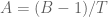 (for some variable
  , which we may want to replace with an exponential) simplifies things quite a bit. For instance, this allows one to convert (2′) into an inequality of the form
  for a function
  (which has a number of nice properties).
20 November, 2013 at 10:05 pm
Pace Nielsen
P.P.S. I just discovered the “FindMaximum” function in Mathematica, which concurs with my findings. When , It says that the RHS of (2) takes a maximum value of
  when (2′) holds, at
  . On the other hand, when
  , then the RHS of (2) is less than 4, when (2′) holds.
If this function is to be believed, when then
then  is the lowest
  value for which the RHS of (2) is bigger than 8 when (2′) also holds. One takes
  .
.
21 November, 2013 at 2:32 am
Andrew Sutherland
The admissible
21 November, 2013 at 1:51 pm
Terence Tao
In light of James’ calculation below that a naive insertion of (or
(or  ) gives good results for the small k numerics, it is now tempting to do the same for the large k asymptotics given above.
If one does things optimistically (ignoring ), then all one has to do is replace the condition
  with
with  for one’s favourite value of
  . Given that in the small k case this improved 105 to 68, perhaps we could hope that 145 improves to below 105?
To do things properly (i.e. rigorously), we unfortunately have to also take into account , and specifically there is an annoying new constraint
needed to ensure that all the moduli involved are -smooth. This (when combined with either
 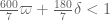 or
or 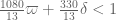 ) is likely to cause some degradation in the bounds, but at least these bounds would be rigorous.
On the other hand, we do know that our MPZ estimates only need a certain amount of dense divisibility rather than smoothness. It is likely that one could modify the above arguments (probably by introducing two different deltas, much as we did in Polymath8a) we could reduce the dependence on delta to the point where it is almost negligible. But this looks a little tricky and is probably best deferred until a little later.
p.s. Gah, I just realised that my formula for given previously was incorrect, as I had lost the
  factor. The true formula for
  is
is
which unfortunately is likely to make the previous computations a little bit worse. Sorry about that!
21 November, 2013 at 2:58 pm
Pace Nielsen
With the corrected formula for , the FindMaximum command gives the following results:
For , we have
  .
.
For , we have
  .
.
I’ll give your other improvement some thought when I have more time.
21 November, 2013 at 4:13 pm
Terence Tao
Thanks for the quick recalculation! It’s a shame that we lost a factor of 5 due to the error, although we still beat Polymath8a, for what it’s worth…
22 November, 2013 at 1:33 am
Andrew Sutherland
With we get
  with this tuple.
21 November, 2013 at 3:51 pm
xfxie
Just had an initial try for . Seems
  cannot be dropped down too far. Here is a possible solution 508.
21 November, 2013 at 8:12 pm
Pace Nielsen
Using , xfxie's
  appears optimal for
  . For
. For  , we can get
  .
.
22 November, 2013 at 6:18 am
Andrew Sutherland
This gives the lower bound 484290 on .
.
22 November, 2013 at 7:04 am
Andrew Sutherland
Of course I meant to say upper bound :)
22 November, 2013 at 7:37 am
Andrew Sutherland
Actually we can get H_2 down to 484276.
22 November, 2013 at 9:18 am
Fan
The link to the 484276 tuple keeps throwing 403
22 November, 2013 at 10:04 am
Andrew Sutherland
Fixed.
23 November, 2013 at 4:13 pm
xfxie
For =42392, seems
  can be further down to 484272 :).
23 November, 2013 at 4:33 pm
Andrew Sutherland
Slight further improvement: 484260.
23 November, 2013 at 6:32 pm
xfxie
Further improved to 484238.
24 November, 2013 at 2:00 am
Andrew Sutherland
Another small improvement: 484234.
24 November, 2013 at 6:35 am
xfxie
Can be further down to 484200.
24 November, 2013 at 6:21 pm
Andrew Sutherland
A little more progress: 484192.
25 November, 2013 at 2:09 am
Andrew Sutherland
484176.
26 November, 2013 at 5:01 am
xfxie
Can be dropped to: 484168 (for k=42392).
27 November, 2013 at 2:08 am
Andrew Sutherland
484162
27 November, 2013 at 12:40 pm
Andrew Sutherland
484142
28 November, 2013 at 4:47 am
Andrew Sutherland
484136
28 November, 2013 at 6:25 am
Andrew Sutherland
484126
20 November, 2013 at 6:36 pm
andre
Please forgive me my ignorance, I even didn’t fully read Maynard’s preprint. with an outer integration over the (k-1)-dim. cube. On page 19, along the proof of Lemma 7.2, formula (7.12) he uses an outer integration over the (k-1)-dim simplex. So my question is, if the outer integration in the definition of
  was over the (k-1)-dim simplex, too?
On page 5, in Proposition 4.1, he defines
20 November, 2013 at 9:13 pm
Terence Tao
In Lemma 7.2, one is only considering functions F of the form defined in (7.3), which are supported on the simplex, and so integration of such functions in the cube is the same as on the simplex.
20 November, 2013 at 6:48 pm
Eytan Paldi
It seems that the largest eigenvalue of the operator defined in (7.2) of Maynard’s preprint is the square root of (not
(not  as remarked there.)
20 November, 2013 at 7:11 pm
Eytan Paldi
In fact, the exact relationship between the above linear operator and is not sufficiently clear to me.
20 November, 2013 at 9:09 pm
Terence Tao
The connection comes from the identity
which shows that is the largest eigenvalue of
  . (Actually, as
  is not quite compact, although it is bounded, self-adjoint, and positive definite, one has to be a little careful here with the spectral theory to ensure that
  only has point spectrum at its operator norm; I think it will work out though, I will try to supply some details later. In any case this doesn’t impact the substance of Maynard’s paper, as one never actually analyses eigenfunctions in that paper.)
20 November, 2013 at 9:37 pm
Eytan Paldi
Thanks for the explanation! One may use this to show that for each given polynomial P, the ratio for should increase (unless P is optimal). This gives iterative process for improving
  .
.
22 November, 2013 at 7:31 am
Terence Tao
A little expansion of Eytan’s remark (a version of the power method): from Cauchy-Schwarz one has
which upon rearranging means that the Rayleigh quotient is non-decreasing if one replaces
  by
by  . Iterating this, we may replace
  by
by  (or any higher power
  and guarantee a better lower bound on
  unless one is already at an eigenfunction.
This suggests that we can improve the large k analysis (and in particular, the m=2 values) by taking our current candidate for f and applying to it to obtain a new candidate that is guaranteed to be better. This is a bit messy though; a simpler (though slightly less efficient) approach would be to compute
  instead of
  and use the inequality
to obtain what should presumably be a better lower bound for M_k than what we currently have.
22 November, 2013 at 8:20 am
Eytan Paldi
In general this iteration gives linear convergence to , so one may try to accelerate it numerically (e.g. by Aitken’s
  method.)
21 November, 2013 at 5:44 am
Eytan Paldi
It seems that the integral operator above is compact since its representing integrand is continuous on its domain (i.e. the product of the simplex in t and the simplex in u.)
But I don’t see why its representing integrand is symmetric (as it should for a self-adjoint operator)!
I suggest to see if the integrands representing powers of this operators can be evaluated explicitly (e.g. by the integrand composition operation) – so the traces of (small) powers of the operator may be evaluated – giving upper bounds for corresponding powers of .
.
21 November, 2013 at 6:57 am
Terence Tao
One can check by hand that for any (say) bounded compactly supported F,G on the simplex.
The operator is not quite an integral operator because each of the
  components only integrates in one of the dimensions rather than all
  of the dimensions. As such, it doesn’t look compact, but may still have pure point spectrum, at least at the top of the spectrum (I have to check this). In particular, I don’t expect the traces of powers of this operator to be finite. A model case here is the operator
 ![T: L^2([0,1]^2) \to L^2([0,1]^2)](https://s0.wp.com/latex.php?latex=T%3A+L%5E2%28%5B0%2C1%5D%5E2%29+%5Cto+L%5E2%28%5B0%2C1%5D%5E2%29&bg=ffffff&fg=545454&s=0&c=20201002) given by
given by
which is positive semi-definite and bounded with an operator norm of 1, but has an infinity of eigenfunctions at 1 (any f that is independent of y will be an eigenfunction).
21 November, 2013 at 7:40 am
Eytan Paldi
Thanks! (I see now my error.)
Anyway, I think that it is also important to get also some upper bounds for (to estimate the tightness of its lower bounds and to get some limitations of the method.)
21 November, 2013 at 11:51 am
Terence Tao
I no longer have any clear intuition as to whether the spectrum of is pure point, absolutely continuous, or some combination of both (it could also possibly have singular continuous spectrum); the situation could be as complicated as it is for discrete or continuous Schrodinger operators, which have a very wide range of possible behaviours. Consider for instance the model operator
on the triangle (all variables are assumed to be non-negative); this is one of the two components of
  in the k=2 case. One can split
  into the functions that are constant in the y direction, and functions that are mean zero in the y direction. The operator T annihilates the latter space, and acts by multiplication by
  on the former space. So there is absolutely continuous spectrum on
 ![[0,1]](https://s0.wp.com/latex.php?latex=%5B0%2C1%5D&bg=ffffff&fg=545454&s=0&c=20201002) and a big null space at 0. The operator norm of 1 is not attained by any function, but one can get arbitrarily close to this norm by, e.g. the indicator function of the rectangle
and a big null space at 0. The operator norm of 1 is not attained by any function, but one can get arbitrarily close to this norm by, e.g. the indicator function of the rectangle ![[0,\varepsilon] \times [0,1-\varepsilon]](https://s0.wp.com/latex.php?latex=%5B0%2C%5Cvarepsilon%5D+%5Ctimes+%5B0%2C1-%5Cvarepsilon%5D&bg=ffffff&fg=545454&s=0&c=20201002) for
for  (one can normalise to have unit norm in L^2 if one wishes).
Despite the possible lack of eigenfunctions (which in particular may mean that in some cases the maximum of the ratio is not attainable), I believe it is still correct that the operator norm of
  for all functions on the simplex is the same as the operator norm of
  for symmetric functions on the simplex, which informally means that we can restrict without loss of generality to the case of symmetric functions F. To see this, suppose that we have a sequence
  of
of  -normalised functions on the simplex which is a extremising sequence for
 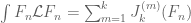 , thus this sequence approaches the supremum
  as
as  . By replacing
  with its absolute value
  (which does not change the L^2 norm, but can only serve to increase the
  ) we may assume that the
  are non-negative. In particular, the projection
  to the symmetric functions (i.e. the symmetrisation of
  ) is bounded away from zero (in fact it is at least
  ). An application of the parallelogram law (or the spectral theorem) shows that any average of two or more extremising sequences is again an extremising sequence (if the norms stay away from zero), so the symmetrised
  are also extremising. (One could also have taken a slightly higher-minded approach and split up
  according to isotypic
  components here if one wished.)
21 November, 2013 at 11:56 am
Terence Tao
My tentative understanding of what is going on near the top of the spectrum is that if one has strict monotonicity then the supremum should be obtained by an eigenfunction of
  , but if one has equality
  then the near-extrema may instead be obtained from lower-dimensional functions, e.g. functions of the form
 ![F(t_1,\ldots,t_k) = F_\varepsilon(t_1,\ldots,t_{k-1}) 1_{[0,\varepsilon]}(t_k)](https://s0.wp.com/latex.php?latex=F%28t_1%2C%5Cldots%2Ct_k%29+%3D+F_%5Cvarepsilon%28t_1%2C%5Cldots%2Ct_%7Bk-1%7D%29+1_%7B%5B0%2C%5Cvarepsilon%5D%7D%28t_k%29&bg=ffffff&fg=545454&s=0&c=20201002) where
where  is a near-extremiser of the
  -dimensional problem (supported on a slightly shrunken version of the
  -dimensional simplex).
It is presumably the case that the are strictly increasing (except possibly for very small k), but I don’t see how one would prove this other than numerically (and even numerical verification is a bit of a challenge because we do not yet have good upper bounds on
  ).
).
22 November, 2013 at 10:49 am
Eytan Paldi
A “steepest descent” type iteration for :
:
Consider the ratio
In a given Hilbert space (in our case
  over the simplex) where L is a linear, symmetric, bounded operator on
  .
.
Clearly, we need to consider whose first variation is
Note that may be interpreted as the “gradient” of
  at x. This implies the “line search” iteration
Where is the direction of search and
 is the search step size (determined to maximize the ratio at
  .
.
Remarks:
1. If is a polynomial then all
  are polynomials.
2. It is easy to find the closed form formula for the search step size.
3. This search can be improved to a “conjugate gradient” type search (and perhaps even to “quasi Newton” type methods) with quadratic convergence rate!
22 November, 2013 at 2:51 pm
Eytan Paldi
It should be remarked that in all iterative methods of this type (i.e. “gradient based”), is a linear combination of
  – for which Maynard’s method (for best linear combination) should be applied on these basis functions.
21 November, 2013 at 4:26 am
Andreas
Shouldn’t that be “where $p_n$ denotes the $n$-th prime” in the beginning?
21 November, 2013 at 5:45 am
Anonymous
I think you are right. Also, I would write “ ”, i.e., with parentheses.
The improvements suggestioned in https://terrytao.wordpress.com/2013/11/19/polymath8b-bounded-intervals-with-many-primes-after-maynard/#comment-251777 could also be incorporated. :)
[Changes now made – T.]
21 November, 2013 at 12:50 pm
James Maynard
One numerical data point that people might find interesting:
Assume![EH[1/4+\varpi]](https://s0.wp.com/latex.php?latex=EH%5B1%2F4%2B%5Cvarpi%5D&bg=ffffff&fg=545454&s=0&c=20201002) with the provisional value
with the provisional value  . Using computations as in my paper (a polynomial approximation of terms
  with
with  , we find for
  that
that 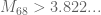 . We find then that
  , and so two primes with
  , which corresponds to gaps of size 356.
21 November, 2013 at 1:08 pm
Terence Tao
That’s smaller than I would have expected, given that is only 5% or so bigger than 1/4. (Incidentally, with our conventions, we would use
 ![EH[2 * (1/4+\varpi) ]](https://s0.wp.com/latex.php?latex=EH%5B2+%2A+%281%2F4%2B%5Cvarpi%29+%5D&bg=ffffff&fg=545454&s=0&c=20201002) rather than
rather than ![EH[1/4+\varpi]](https://s0.wp.com/latex.php?latex=EH%5B1%2F4%2B%5Cvarpi%5D&bg=ffffff&fg=545454&s=0&c=20201002) . But I guess since
. But I guess since  is already as large as 2, and
  seems to grow logarithmically, it isn’t so unreasonable.
Do you have some preliminary data on how your lower bounds on behave in k for small k (e.g. up to 105)? This would give a baseline for further numerical improvement, and would also give a better sense as to what kind of growth
  should have (given that the values should be pretty good for small k, perhaps enough to do some reliable extrapolation).
Of course we have to play with MPZ instead of EH, which causes some difficulties (specifically, we can’t play on the entire simplex, but must truncate to the cube![[0, \frac{\delta}{1/4+\varpi}]^k](https://s0.wp.com/latex.php?latex=%5B0%2C+%5Cfrac%7B%5Cdelta%7D%7B1%2F4%2B%5Cvarpi%7D%5D%5Ek&bg=ffffff&fg=545454&s=0&c=20201002) ), but it does show that there is hopefully a fair bit of room for improvement.
), but it does show that there is hopefully a fair bit of room for improvement.
Incidentally, the 7/600 value is not so provisional (once Emmanuel signs off on Section 10 of the Polymath8a paper, in particular, it would have been checked at least once). We have a much more tentative value of 13/1080 that is not fully verified (it requires some difficult algebraic geometry that we haven’t got around to yet) but it might be interesting to see how much more of a gain one could expect with this slightly better value.
21 November, 2013 at 4:10 pm
James Maynard
The growth looks roughly logarithmic.
A reasonable approximation for is
is  .Specifically, for
 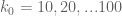 I get the following bounds: 2.53, 3.05, 3.34, 3.52, 3.66, 3.76, 3.84, 3.90, 3.95, 3.99.
21 November, 2013 at 1:27 pm
Stijn Hanson
Sorry for the stupid question but, In Maynard’s Lemma 5.1 (and roughly in here just below (10) ) it states that if![W, [d_1, e_1], \ldots, [d_k, e_k]](https://s0.wp.com/latex.php?latex=W%2C+%5Bd_1%2C+e_1%5D%2C+%5Cldots%2C+%5Bd_k%2C+e_k%5D&bg=ffffff&fg=545454&s=0&c=20201002) are not pairwise coprime then
are not pairwise coprime then  and
and ![[d_i,e_i]|n+h_i](https://s0.wp.com/latex.php?latex=%5Bd_i%2Ce_i%5D%7Cn%2Bh_i&bg=ffffff&fg=545454&s=0&c=20201002) cannot be satisfied by any n. It’s utterly trivial if d divides n and one of the lcms but I can’t seem to understand why it works if d divides two of the lcms.
cannot be satisfied by any n. It’s utterly trivial if d divides n and one of the lcms but I can’t seem to understand why it works if d divides two of the lcms.
21 November, 2013 at 4:23 pm
Terence Tao
If d divides both![[d_i,e_i]](https://s0.wp.com/latex.php?latex=%5Bd_i%2Ce_i%5D&bg=ffffff&fg=545454&s=0&c=20201002) and
and ![[d_j,e_j]](https://s0.wp.com/latex.php?latex=%5Bd_j%2Ce_j%5D&bg=ffffff&fg=545454&s=0&c=20201002) , then it divides
, then it divides  and
and  , and hence also
  . On the other hand, since
  is coprime to W,
  must be coprime to
  . Since
  is the product of all small primes, and in particular all primes dividing
  (if x is large enough), we obtain a contradiction.
22 November, 2013 at 8:30 am
Terence Tao
I think there is a probabilistic interpretation of M_k, as follows. Consider the following random process![x^{(0)}, x^{(1)}, \ldots \in [0,1]^k](https://s0.wp.com/latex.php?latex=x%5E%7B%280%29%7D%2C+x%5E%7B%281%29%7D%2C+%5Cldots+%5Cin+%5B0%2C1%5D%5Ek&bg=ffffff&fg=545454&s=0&c=20201002) on the unit cube as follows:
on the unit cube as follows:
* is chosen uniformly at random from the unit cube.
* Once is chosen,
  is chosen by taking
  , selecting a random coordinate of
  , and replacing it with a number chosen uniformly from [0,1] independently of all previous choices.
(For the chess-oriented, this process describes a (k-dimensional) rook moving randomly in the unit cube.)
The probability that all lie in the simplex is
  , which asymptotically is
 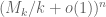 as
as  . So
. So  is measuring the exponential decay of the probability that the randomly moving rook always stays inside the simplex.
Among other things, this suggests that a Monte Carlo method might be used to approximate , although this would not give rigorous deterministic bounds on
  .
.
24 January, 2014 at 9:37 am
Eytan Paldi
Is it possible to give to a quantum mechanical interpretation as well? (The problem is to give a quantum mechanical interpretation to the operator
  – which may make sense in smaller dimensions like 3,4).
 ?
?
Perhaps quantum mechanical bounds (a kind of “uncertainty principle”) bounds may be obtained for
22 November, 2013 at 10:11 am
Terence Tao
Here are my (unfortunately somewhat lengthy) computations for the second moment for the function
used in the large k analysis, with the quantities defined in this previous comment. Note that
  , and hence
and
so we can get lower bounds on by computing either of the quantities in (1) and (2), and we know from Cauchy-Schwarz that (2) should give a slightly better bound.
As a warmup, let us first compute the RHS of (1). By symmetry, this becomes
which if we restrict to the region , simplifies to
where are iid with distribution
  on
on ![[0,T]](https://s0.wp.com/latex.php?latex=%5B0%2CT%5D&bg=ffffff&fg=545454&s=0&c=20201002) . This, together with the Chebyshev inequality, is what gives the lower bound
. This, together with the Chebyshev inequality, is what gives the lower bound
which is what we had in the previous comment.
Now we compute the RHS of (2). By symmetry, this becomes the sum of
and
For the first expression, we restrict to the region and obtain a lower bound of
By Chebyshev, this is at least
subject to the constraint
Meanwhile,for the second expression we restrict to the region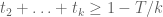 and obtain a lower bound of
which we can lower bound by
which is equal to
Thus we obtain the bound
whenever obey the constraint (4).
Asymptotically, this does not seem to give too much of an improvement to the lower bound of (a back of the envelope calculation suggests that the gain is only
  or less) but it might still give some noticeable improvement for the m=1 and m=2 numerics. (And if it doesn’t, it would provide some indication as to how close our test function F is to being an eigenfunction.)
22 November, 2013 at 1:47 pm
Pace Nielsen
Is your formula for (3) correct? Or should there be a square in the denominator of the rightmost fraction? [I ask, because three offset equations earlier, you have a formula that doesn’t match your earlier bound for as it it missing a square in the denominator of the rightmost fraction as well.]
22 November, 2013 at 1:52 pm
Terence Tao
Yes, you’re right; there should be a square in the denominator in both cases as per Chebyshev. So the first lower bound for M_k should be
and the quantity in (3) should instead be
Thanks for spotting the error. But actually this error may end up in our favour, since I think the denominator is in fact greater than 1, so perhaps xfxie’s calculations below will in fact improve with this correction!
22 November, 2013 at 2:03 pm
Pace Nielsen
Unfortunately (or fortunately, depending on your frame of reference) xfxie’s calculation used the correct formula. When I wasn’t able to reproduce his results, I discovered the error.
22 November, 2013 at 3:03 pm
xfxie
Pace is right. For the implementation, I modified the code based on the obvious difference between M_k and (3) — so it might be the reason that the typo (which appeared in both places) was automatically skipped.
22 November, 2013 at 2:01 pm
Pace Nielsen
Assuming that the answer to my question is that the formula for (3) was incorrect, and that there should be a square (which I think is true, if I’m understanding your use of Chebyshev), we get (without using the inequalities from Polymath 8a) the following:
For ,
,  .
. ,
,  .
. .
.
For
Under EH,
23 November, 2013 at 1:28 am
Andrew Sutherland
This implies is at most 493528.
23 November, 2013 at 10:23 am
Andrew Sutherland
Actually, this can be improved slightly: 493510
23 November, 2013 at 4:40 pm
Andrew Sutherland
Further improved to 493458.
24 November, 2013 at 6:16 pm
Andrew Sutherland
Down to 493442.
25 November, 2013 at 1:53 pm
Andrew Sutherland
493436
26 November, 2013 at 1:53 am
Andrew Sutherland
493426
6 December, 2013 at 7:32 am
Andrew Sutherland
493408
22 November, 2013 at 5:07 pm
Terence Tao
I’m noting a rather technical complication with this second moment computation when one tries to combine it with![MPZ[\varpi,\delta]](https://s0.wp.com/latex.php?latex=MPZ%5B%5Cvarpi%2C%5Cdelta%5D&bg=ffffff&fg=545454&s=0&c=20201002) . When using MPZ, one has effectively limited oneself to using functions
. When using MPZ, one has effectively limited oneself to using functions  supported on the cube
 ![[0, \frac{\delta}{1/4+\varpi}]^k](https://s0.wp.com/latex.php?latex=%5B0%2C+%5Cfrac%7B%5Cdelta%7D%7B1%2F4%2B%5Cvarpi%7D%5D%5Ek&bg=ffffff&fg=545454&s=0&c=20201002) to get smoothness of the moduli. However, while the original function f has this form (if
to get smoothness of the moduli. However, while the original function f has this form (if  ), higher iterates
  do not necessarily have this form. So, strictly speaking, one cannot combine the two improvements.
However, this is likely a fixable problem provided one puts in a certain amount of effort. The function is still supported on a set in which all but m of the coordinates are known to lie in
 ![[0, \frac{\delta}{1/4+\varpi}]^k](https://s0.wp.com/latex.php?latex=%5B0%2C+%5Cfrac%7B%5Cdelta%7D%7B1%2F4%2B%5Cvarpi%7D%5D%5Ek&bg=ffffff&fg=545454&s=0&c=20201002) , which for small m almost guarantees multiple
, which for small m almost guarantees multiple  -dense divisibility, if not
  -smoothness (there will be an exceptional set in which this fails but it will be exponentially small). So it is likely that this technicality will have a negligible impact on the estimates, and hopefully will not degrade the value of k at all.
It’s all getting rather complicated; I will try to write up a fresh blog post soon to summarise the various things being explored here.
22 November, 2013 at 11:17 am
xfxie
For , seems
  can drop significantly. Here is a possible solution 388, if my implementation is correct.
22 November, 2013 at 12:54 pm
Aubrey de Grey
xfxie, can you please clarify – which permutation of other assumptions are you using here? Or to put it another way, to which previously-mentioned k0 assuming varpi = 7/600 (if any) is your 388 the 13/1080 counterpart?
22 November, 2013 at 3:13 pm
xfxie
Aubery, 13/1080 is based on Terence’s calculation here (and the counterpart of k_0 is 603). It is also mentioned in an comment above by Terence. The result is not totally verified yet. But the calculation might provide a basic sense on how far the method can reach.
24 November, 2013 at 12:05 pm
Aubrey de Grey
Thanks, but actually that wasn’t quite my question: I know that 603 is the pre-Maynard k0 for varpi = 13/1080, but I was looking for the post-Maynard k0 for varpi = 7/600. If I’m not mistaken, Pace’s k0 of 448 assumes only Bombieri-Vinogradov, and until 13/1080 is fully confirmed I’m thinking that it might be of interest also to continue tracking the various k0 that arise from 7/600.
Also, incidentally, isn’t k0 = 42392 obsolete now? – isn’t that the m=2 counterpart of 508, which was superseded by Terry’s second-moment computations on Friday? I’m unclear as to why you and Drew are still refining H for 42392 rather than for the m=2 counterpart of 388 (which I don’t think anyone has posted yet).
24 November, 2013 at 6:35 pm
Andrew Sutherland
The situation with k0=42392 isn’t clear to me, but if someone has a better value, please post it; I agree there is no point in optimizing H values for an obsolete k0 (although it has motivated me to spend some time tweaking the algorithm to more efficiently handle k0 in this range, so the time isn’t wasted). I’d also be curious to see a k0 for m=3 if anyone is motivated enough to try it.
As far as I know the best “Deligne-free” k0 for m=2 is still 43134, but someone please correct me if I am wrong.
22 November, 2013 at 2:04 pm
Terence Tao
I think I now have an upper bound of of logarithmic type that matches the lower bound asymptotically (up to the
  correction terms).
First, let me describe the warmup problem which led me to discover the bound. Morally speaking (ignoring the terms), the large k computations boil down to the problem of maximising
  subject to the constraints
  and
and  . Calculus of variations tells us that the extremiser should be a multiple of
  for some suitable
  . Motivated by this, I wrote down the Cauchy-Schwarz inequality
(knowing that equality is attained here when is a multiple of
  ) and the right-hand side evaluates to be bounded by
which optimises to essentially (up to errors of
  ) after setting
  (say).
This then led me to an analogous argument in the multidimensional setting (after a rescaling). Namely, Cauchy-Schwarz gives
The latter integral evaluates to . Integrating in the remaining variables
  , we conclude that
Similarly for permutations. Summing and using the fact that on the simplex, we conclude that
and so we have the upper bound
for any ; again setting
  , we obtain an upper bound of the form
and one can probably optimise this a bit further.
22 November, 2013 at 3:05 pm
Eytan Paldi
For small , this is quite close to Maynard’s lower bounds logarithmic approximation above.
2 April, 2014 at 7:28 am
Gergely Harcos
Just a very small note that the term can be taken as
  for all
  .
.
22 November, 2013 at 2:23 pm
Eytan Paldi
It seems that it should be “…multiple of …”.
…”.
[Corrected, thanks – T.]
22 November, 2013 at 2:28 pm
Eytan Paldi
Sorry, at first sight it seems to me (instead of its inverse.)
22 November, 2013 at 2:28 pm
Pace Nielsen
Minor typo: Eight lines from the bottom, should be
  .
.
[Actually, I think it is correct as it stands, although I had skipped a step involving cancelling a factor of which I have now put back in to try to reduce confusion. -T.]
22 November, 2013 at 5:36 pm
Pace Nielsen
You are right. Sorry about that!
22 November, 2013 at 7:41 pm
Polymath8b, II: Optimising the variational problem and the sieve | What's new
[…] for small values of (in particular ) or asymptotically as . The previous thread may be found here. The currently best known bounds on […]
22 November, 2013 at 7:44 pm
Terence Tao
Rolling over the thread to a fresh one in order to make it easier to catch up on the discussion.
23 November, 2013 at 2:27 am
Nikita Sidorov
Out of curiosity – what does the numerics suggest for $H_m$?
27 November, 2013 at 6:59 am
Primzahlenzwillinge | UGroh's Weblog
[…] Artikel in dem Quanta Magazin findet man mehr über die neusten Entwicklungen dazu (siehe auch den Blog von Terence Tao […]
7 December, 2013 at 4:06 pm
Ultraproducts as a Bridge Between Discrete and Continuous Analysis | What's new
[…] transfer from the corresponding laws for the standard natural numbers . For a more topical example, it is now a theorem that given any standard natural number , there exist standard primes such that ; it is an […]
8 December, 2013 at 4:47 pm
Polymath8b, III: Numerical optimisation of the variational problem, and a search for new sieves | What's new
[…] the notation of this previous post, we have the lower […]
20 December, 2013 at 2:05 pm
Polymath8b, IV: Enlarging the sieve support, more efficient numerics, and explicit asymptotics. | What's new
[…] products supported on small cubes in avoiding (5). For the GPY argument to work (as laid out in this previous post), we need the […]
8 January, 2014 at 11:21 am
Polymath8b, V: Stretching the sieve support further | What's new
[…] baseline bounds for the numerator and denominator in (1) (as established for instance in this previous post) are as follows. If is supported on the […]
28 January, 2014 at 9:19 pm
Polymath8b, VII: Using the generalised Elliott-Halberstam hypothesis to enlarge the sieve support yet further | What's new
[…] wish to understand the correlation of various products of divisor sums on . For instance, in this previous blog post, the […]
2 February, 2014 at 3:44 pm
Коллективный разум в теории чисел » CreativLabs
[…] растерялся и огранизовал новый коллективный проект polymath8b, направленный на улучшение вновь полученной границы. […]
2 February, 2014 at 6:43 pm
Eytan Paldi
On the dependence of the current M-value on :
:
According to some preliminary analysis, it seems that for , we have the linear dependence
For some (still undetermined) absolute positive constant C (related to the solution of a certain integral equation). Interestingly, it is easy to determine the dependence on without knowing the constant C!
I suggest to verify empirically this linear dependence.
14 March, 2014 at 11:17 am
Urns and the Dirichlet Distribution | Eventually Almost Everywhere
[…] Polymath8b: Bounded intervals with many primes, after Maynard (terrytao.wordpress.com) […]
1 April, 2014 at 10:42 am
Gergely Harcos
I think that (8) in Proposition 7 is valid for all , not just for
  sufficiently large. First, we can assume that
  , since otherwise the right hand side of (8) is negative. Then, in the bound (8.17) of Maynard’s paper, we can choose
  such that
  . Clearly,
  , i.e.
  . In addition, on the right hand side of (8.17),
  and
and  .
.  is less than
  , hence the right hand side of (8.17) exceeds
  , which in turn is greater than
  .
.
31 July, 2014 at 8:33 am
Together and Alone, Closing the Prime Gap | For a better Vietnam
[…] However, Tao predicted that the project’s participants will not be able to resist immediately sinking their teeth into Maynard’s new preprint. “It’s like red meat,” he […]
6 December, 2015 at 2:23 am
Anonymous
Why we need to choose the simplex such? What to change if you take $R_k=\{\dots(x)\in[0,1]^k\}$?
6 December, 2015 at 4:28 pm
Terence Tao
The restriction to the simplex is needed to force the products and
and  to be bounded by
  (see second display before (11)), which is in turn needed in order to have good equidistribution estimates available (with error term smaller than the main term).
21 March, 2016 at 9:49 am
Anonymous
If you apply the approach of Maynard to , then to assess the difference
  we must demand
  . But
. But  . Choosing N large enough, we achieve the minimum distance for any r, which obviously leads to a contradiction. Where am I wrong?
[Wordpress treats < and > as HTML, causing text with both symbols in it to be corrupted. Use < and > instead – T.]
26 May, 2016 at 8:45 am
Anonymous
Where in the proof of the asymptotics for sums (10),(11) significantly that the set is admissible? Thanks.
26 May, 2016 at 9:07 am
Terence Tao
One needs admissibility in order to have at least one residue class with all of the
  coprime to
  . So estimates such as (1) and (2) are vacuously true in the non-admissible case (because there is no
  that obeys the requirements).
26 May, 2016 at 10:33 am
Anonymous
Is it possible to formulate the allowed set is defined for arbitrary subsets of natural numbers? For example, if we consider the set of Prime numbers,the distance between which is greater than 1000, then the asymptotic amount and level of distribution will not change. Then, using Your approach, we would have the presence of smaller distances of 600 and would come to a contradiction. This is due to the choice of the set H. We knew in advance that, for example, n and n+2 could not lie simultaneously in our set and therefore had no right to choose so.
26 May, 2016 at 10:39 am
Terence Tao
I’m not fully sure I understand your question, but this method has been extended to find small gaps in other sets of numbers than the primes, see e.g. the work of Benatar, Thorner, Li-Pan, Pollack, Maynard, Chua-Park-Smith, and Baker-Zhao (this may not be a complete list of references).
17 June, 2016 at 5:13 am
Anonymous
Good afternoon!
Take the set of primes p such that p+2 and p-2 is obviously not a prime number. The asymptotic number of integers in this set and the level of distribution are the same as primes. Can we apply to this set the approach of Maynard? Thank you!
18 June, 2016 at 7:22 am
Terence Tao
It depends on what you mean by “obviously”. If you mean that and
and  are each divisible by some small prime (e.g. 3 and 5 respectively), then as you say one has the required level of distribution, and it is not difficult to adapt the arguments (there are already several papers in the literature dealing with bounded gaps between special sets of primes obeying these sorts of level of distribution axioms). But if you only require that
  are both composite, then a level of distribution result (with error terms that are better than the main terms by an arbitrary power of
  ) would basically require the conjectural asymptotics for the twin prime conjecture, which is of course still open.
19 June, 2016 at 2:32 pm
Anonymous
Could You provide a link to the literature?
20 June, 2016 at 7:35 am
Terence Tao
See my previous comment on this blog post at 2016/05/26 at 10:39 am.
20 February, 2017 at 4:19 am
Anonymous
What is known about such sums with weights fourth degree or more? Why we study a second degree? Thank you.
20 February, 2017 at 10:04 am
Anonymous
It seems that fourth degree weights should have narrower peaks (i.e. more selective) which is somewhat analogous to Jackson kernel (fourth degree weights) versus Fejer kernel (second degree weights) in approximation theory.
24 February, 2017 at 11:10 am
Anonymous
Where I could read more about it? I tried to bring the corresponding coefficients of the main parts, and got unexpectedly complicated structure.
25 February, 2017 at 8:55 am
Anonymous
The idea to use such weights already appeared in a comment (10 August, 2014, at 11:38 am) in the 36-th Polymath8 thread (from 21 July 2014).
20 February, 2017 at 3:08 pm
sylvainjulien
Assuming Goldbach’s conjecture, and denoting by $ latex r_{0}(n) $ the smallest positive integer $ latex r $ such that both $ latex n-r $ and $ latex n+r $ are primes for latex n$ a large enough composite integer, and by $ latex l0(n) $ the number of primes in the interval $ latex [n-r_{0}(n),n+r_{0}(n)] $ , what would be the best upper bound for $ latex l_{0}(n) $ in terms of $ latex r_{0}(n) $ ? Can $ latex l_{0}(n)\ll_{h} (r_{0}(n))^{1/2+h} $ hold true under GRH ?
26 February, 2017 at 9:30 am
Anonymous
Dear Terry,
Could you please answer the following question: if we consider the weight of the fourth degree, the values will look like as in the second degree with the exception of the degree of
  ? I used the Fourier transform method and received a rather complex structure. So I’m trying to understand if I have a mistake.
Thank you!
11 March, 2017 at 8:50 am
Anonymous
What restrictions need to require the function to compute values
  and
and  in the original form (5),(6)?
 then
then  Where am I making a mistake?
For example, if we take
15 March, 2017 at 9:44 pm
Terence Tao
This function is not supported on the simplex (and if one truncates the function to this simplex, it will no longer be smooth).
15 March, 2017 at 11:24 pm
Anonymous
Then which function to choose?
12 March, 2017 at 1:53 pm
sylvainjulien
Dear Terry,
Can an interesting lower bound for the de Polignac constant as introduced in http://math.stackexchange.com/questions/2183872/lower-bound-for-the-de-polignac-constant be obtained as of today (March 12th 2017) ?
Many thanks in advance.
3 October, 2020 at 4:38 pm
Hoa Huynh
Assuming the GEH, the bounded gap is 6.
In Wikipedia of “Polignac’s conjecture”, in section “Conjectured density”, there is a statement:
Twin primes have the same conjectured density as cousin primes, and half that of sexy primes.
Together, don’t they imply that all 3: Twin Prime, Cousin Prime and Sexy Prime have infinite counts?
4 October, 2020 at 5:27 pm
Terence Tao
Conjecturally, yes. But this is not yet proven.
5 October, 2020 at 5:57 am
sylvainjulien
You may be interested in this: https://mathoverflow.net/questions/358027/a-conditional-approach-to-twin-prime-conjecture?r=SearchResults
6 October, 2020 at 6:52 am
Hoa Huynh
For “admissible tuples”, the first element’s position or pattern is fixed for “k equal to or greater than 6.”
Examples:
For k = 5, we have 2 patterns: (p, p + 2, p + 6, p + 8, p + 12)
16061, 16063, 16067, 16069, 16073 (*)
21011, 21013, 21017, 21019, 21023
43781, 43783, 43787, 43789, 43793 (*)
247601, 247603, 247607, 247609, 247613
1063961, 1063963, 1063967, 1063969, 1063973
1091261, 1091263, 1091267, 1091269, 1091273 (*)
1246361, 1246363, 1246367, 1246369, 1246373
and (p, p + 4, p + 6, p + 10, p + 12)
15727, 15731, 15733, 15737, 15739
16057, 16061, 16063, 16067, 16069 (*)
43777, 43781, 43783, 43787, 43789 (*)
79687, 79691, 79693, 79697, 79699
736357, 736361, 736363, 736367, 736369
1091257, 1091261, 1091263, 1091267, 1091269 (*)
1155607, 1155611, 1155613, 1155617, 1155619
——–
For k = 6, we have 1 pattern: (p, p + 4, p + 6, p + 10, p + 12, p + 16)
16057, 16061, 16063, 16067, 16069, 16073 (*)
43777, 43781, 43783, 43787, 43789, 43793 (*)
1091257, 1091261, 1091263, 1091267, 1091269, 1091273 (*)
——–
There are many many more of them, the examples are chosen to illustrate the points: pattern for k = 6 exists in k = 5; and the 4 middle elements are in the same decade, and the 2 outside ones are in adjacent decades.
The unit digits for k = 6 are fixed: 7, 1, 3, 7, 9, 3. The obvious reason is to avoid divisibility by 5.
Likewise, “fixed unit digit patterns” also happen for k > 6, for “optimal sieving.”
——–
Has this information/fact been used in some proofs of bounded gap?
8 October, 2020 at 7:44 am
Hoa Huynh
For the 105-tuple, we can not place its FIRST element at even-numbered locations, because it sieves all even numbers.
It has 26 numbers ended with 0, let’s call it group A. We would NOT place it at locations ended with 5, because we waste 25% of the “resource.”
Group A (26 counts)
0, 10, 30, 70, 90, 100,
120, 180, 190,
220, 250, 280,
300, 310, 330, 360,
390, 400, 420, 430, 450,
490, 510,
570, 580, 600
——————-
Let’s group the rest of 105-tuple in numbers ended with 2, 4, 6 and 8. Note that we don’t have any number ended with 6. So, we have 3 more groups B, C and D, as followed.
Group B (27 counts)
12, 42, 52, 72, 82,
112, 132,
192, 202, 222, 232, 252, 262,
322, 342, 352, 372,
402, 412, 432, 442,
462, 472, 492, 532,
562, 582
—–
Group C (27 counts)
24, 34, 54, 64, 94,
114, 124, 154, 174, 184,
204, 234, 264,
294, 324, 334, 364,
384, 394, 444,
454, 484, 504, 534,
544, 574, 594
——-
Group D (25 counts)
28, 48, 78,
118, 138, 148, 168, 178,
208, 258, 268,
288, 328, 358,
378, 408, 418,
468, 478, 498, 528, 538,
558, 588, 598
—————————
We would not place FIRST element of 105-tuple at locations ended with 3, because group B would waste 25% of the “resource.”
Likewise, for locations ended with 1 and 7, for groups C and D, respectively.
—————————
Therefore, the most strategic locations to place 105-tuple are where they are ended with 9, in order to maximize the result.
Same reason for all k-tuples, with k > 6.
26 January, 2023 at 10:48 am
Infinite partial sumsets in the primes | What's new
[…] that powers the proof of that theorem (though we use a formulation of that sieve closer to that in this blog post of mine). Indeed, the failure of (iii) basically arises from the failure of Maynard’s theorem for […]
1 February, 2023 at 4:07 pm
Infinite partial sumsets in the primes – Terence Tao – A2Z Facts
[…] that powers the proof of that theorem (though we use a formulation of that sieve closer to that in this blog post of mine). Indeed, the failure of (iii) basically arises from the failure of Maynard’s theorem for dense […]