Suppose one is given a  -tuple
  of distinct integers for some
  , arranged in increasing order. When is it possible to find infinitely many translates
  of
of  which consists entirely of primes? The case
  is just Euclid’s theorem on the infinitude of primes, but the case
  is already open in general, with the
  case being the notorious twin prime conjecture.
On the other hand, there are some tuples for which one can easily answer the above question in the negative. For instance, the only translate of  that consists entirely of primes is
  , basically because each translate of must contain an even number, and the only even prime is
  . More generally, if there is a prime
  such that meets each of the residue classes
  , then every translate of contains at least one multiple of ; since is the only multiple of that is prime, this shows that there are only finitely many translates of that consist entirely of primes.
To avoid this obstruction, let us call a -tuple admissible if it avoids at least one residue class  for each prime . It is easy to check for admissibility in practice, since a -tuple is automatically admissible in every prime larger than , so one only needs to check a finite number of primes in order to decide on the admissibility of a given tuple. For instance,
  or
or  are admissible, but
  is not (because it covers all the residue classes modulo
  ). We then have the famous Hardy-Littlewood prime tuples conjecture:
Conjecture 1 (Prime tuples conjecture, qualitative form) If is an admissible -tuple, then there exists infinitely many translates of that consist entirely of primes.
This conjecture is extremely difficult (containing the twin prime conjecture, for instance, as a special case), and in fact there is no explicitly known example of an admissible -tuple with  for which we can verify this conjecture (although, thanks to the recent work of Zhang, we know that
  satisfies the conclusion of the prime tuples conjecture for some
  , even if we can’t yet say what the precise value of
  is).
is).
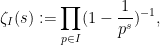
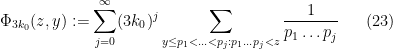
Actually, Hardy and Littlewood conjectured a more precise version of Conjecture 1. Given an admissible -tuple , and for each prime , let  denote the number of residue classes modulo that meets; thus we have
  for all by admissibility, and also
  for all
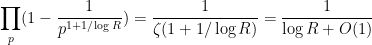
  . We then define the singular series
  associated to by the formula
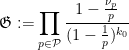
where  is the set of primes; by the previous discussion we see that the infinite product in
  converges to a finite non-zero number.
We will also need some asymptotic notation (in the spirit of “cheap nonstandard analysis“). We will need a parameter  that one should think of going to infinity. Some mathematical objects (such as and ) will be independent of and referred to as fixed; but unless otherwise specified we allow all mathematical objects under consideration to depend on . If
  and
and  are two such quantities, we say that
  if one has
  for some fixed
  , and
, and  if one has
  for some function
  of (and of any fixed parameters present) that goes to zero as
  (for each choice of fixed parameters).
Conjecture 2 (Prime tuples conjecture, quantitative form) Let be a fixed natural number, and let be a fixed admissible -tuple. Then the number of natural numbers  such that
  consists entirely of primes is
  .
.
Thus, for instance, if Conjecture 2 holds, then the number of twin primes less than should equal  , where
  is the twin prime constant
As this conjecture is stronger than Conjecture 1, it is of course open. However there are a number of partial results on this conjecture. For instance, this conjecture is known to be true if one introduces some additional averaging in ; see for instance this previous post. From the methods of sieve theory, one can obtain an upper bound of  for the number of with
  all prime, where
  depends only on . Sieve theory can also give analogues of Conjecture 2 if the primes are replaced by a suitable notion of almost prime (or more precisely, by a weight function concentrated on almost primes).
Another type of partial result towards Conjectures 1, 2 come from the results of Goldston-Pintz-Yildirim, Motohashi-Pintz, and of Zhang. Following the notation of this recent paper of Pintz, for each  , let
, let ![{DHL[k_0,2]}](https://s0.wp.com/latex.php?latex=%7BDHL%5Bk_0%2C2%5D%7D&bg=ffffff&fg=000000&s=0&c=20201002) denote the following assertion (DHL stands for “Dickson-Hardy-Littlewood”):
denote the following assertion (DHL stands for “Dickson-Hardy-Littlewood”):
Conjecture 3 () Let be a fixed admissible -tuple. Then there are infinitely many translates of which contain at least two primes.
This conjecture gets harder as gets smaller. Note for instance that ![{DHL[2,2]}](https://s0.wp.com/latex.php?latex=%7BDHL%5B2%2C2%5D%7D&bg=ffffff&fg=000000&s=0&c=20201002) would imply all the cases of Conjecture 1, including the twin prime conjecture. More generally, if one knew for some , then one would immediately conclude that there are an infinite number of pairs of consecutive primes of separation at most
would imply all the cases of Conjecture 1, including the twin prime conjecture. More generally, if one knew for some , then one would immediately conclude that there are an infinite number of pairs of consecutive primes of separation at most  , where is the minimal diameter
  amongst all admissible -tuples . Values of for small can be found at this link (with denoted
  in that page). For large , the best upper bounds on have been found by using admissible -tuples of the form

where  denotes the
  prime and
  is a parameter to be optimised over (in practice it is an order of magnitude or two smaller than ); see this blog post for details. The upshot is that one can bound for large by a quantity slightly smaller than
  (and the large sieve inequality shows that this is sharp up to a factor of two, see e.g. this previous post for more discussion).
In a key breakthrough, Goldston, Pintz, and Yildirim were able to establish the following conditional result a few years ago:
Theorem 4 (Goldston-Pintz-Yildirim) Suppose that the Elliott-Halberstam conjecture ![{EH[\theta]}](https://s0.wp.com/latex.php?latex=%7BEH%5B%5Ctheta%5D%7D&bg=ffffff&fg=000000&s=0&c=20201002) is true for some
is true for some  . Then is true for some finite . In particular, this establishes an infinite number of pairs of consecutive primes of separation
  .
.
The dependence of constants between and  given by the Goldston-Pintz-Yildirim argument is basically of the form
  . (UPDATE: as recently observed by Farkas, Pintz, and Revesz, this relationship can be improved to
  .)
.)
Unfortunately, the Elliott-Halberstam conjecture (which we will state properly below) is only known for  , an important result known as the Bombieri-Vinogradov theorem. If one uses the Bombieri-Vinogradov theorem instead of the Elliott-Halberstam conjecture, Goldston, Pintz, and Yildirim were still able to show the highly non-trivial result that there were infinitely many pairs
  of consecutive primes with
  (actually they showed more than this; see e.g. this survey of Soundararajan for details).
Actually, the full strength of the Elliott-Halberstam conjecture is not needed for these results. There is a technical specialisation of the Elliott-Halberstam conjecture which does not presently have a commonly accepted name; I will call it the Motohashi-Pintz-Zhang conjecture ![{MPZ[\varpi]}](https://s0.wp.com/latex.php?latex=%7BMPZ%5B%5Cvarpi%5D%7D&bg=ffffff&fg=000000&s=0&c=20201002) in this post, where
in this post, where  is a parameter. We will define this conjecture more precisely later, but let us remark for now that is a consequence of
 ![{EH[\frac{1}{2}+2\varpi]}](https://s0.wp.com/latex.php?latex=%7BEH%5B%5Cfrac%7B1%7D%7B2%7D%2B2%5Cvarpi%5D%7D&bg=ffffff&fg=000000&s=0&c=20201002) .
.
We then have the following two theorems. Firstly, we have the following strengthening of Theorem 4:
Theorem 5 (Motohashi-Pintz-Zhang) Suppose that is true for some . Then is true for some .
A version of this result (with a slightly different formulation of ) appears in this paper of Motohashi and Pintz, and in the paper of Zhang, Theorem 5 is proven for the concrete values  and
and  . We will supply a self-contained proof of Theorem 5 below the fold, the constants upon those in Zhang’s paper (in particular, for , we can take as low as
  , with further improvements on the way). As with Theorem 4, we have an inverse quadratic relationship
  .
.
In his paper, Zhang obtained for the first time an unconditional advance on :
Theorem 6 (Zhang) is true for all  .
.
This is a deep result, building upon the work of Fouvry-Iwaniec, Friedlander-Iwaniec and Bombieri–Friedlander–Iwaniec which established results of a similar nature to but simpler in some key respects. We will not discuss this result further here, except to say that they rely on the (higher-dimensional case of the) Weil conjectures, which were famously proven by Deligne using methods from l-adic cohomology. Also, it was believed among at least some experts that the methods of Bombieri, Fouvry, Friedlander, and Iwaniec were not quite strong enough to obtain results of the form , making Theorem 6 a particularly impressive achievement.
Combining Theorem 6 with Theorem 5 we obtain for some finite ; Zhang obtains this for but as detailed below, this can be lowered to  . This in turn gives infinitely many pairs of consecutive primes of separation at most . Zhang gives a simple argument that bounds
  by
by  , giving his famous result that there are infinitely many pairs of primes of separation at most ; by being a bit more careful (as discussed in this post) one can lower the upper bound on to
  , and if one instead uses the newer value for one can instead use the bound
  . (Many thanks to Scott Morrison for these numerics.) UPDATE: These values are now obsolete; see this web page for the latest bounds.
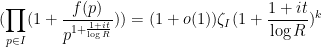
In this post we would like to give a self-contained proof of both Theorem 4 and Theorem 5, which are both sieve-theoretic results that are mainly elementary in nature. (But, as stated earlier, we will not discuss the deepest new result in Zhang’s paper, namely Theorem 6.) Our presentation will deviate a little bit from the traditional sieve-theoretic approach in a few places. Firstly, there is a portion of the argument that is traditionally handled using contour integration and properties of the Riemann zeta function; we will present a “cheaper” approach (which Ben Green and I used in our papers, e.g. in this one) using Fourier analysis, with the only property used about the zeta function  being the elementary fact that blows up like
  as one approaches
  from the right. To deal with the contribution of small primes (which is the source of the singular series ), it will be convenient to use the “
 -trick” (introduced in this paper of mine with Ben), passing to a single residue class mod (where is the product of all the small primes) to end up in a situation in which all small primes have been “turned off” which leads to better pseudorandomness properties (for instance, once one eliminates all multiples of small primes, almost all pairs of remaining numbers will be coprime).
— 1. The -trick —
In this section we introduce the “-trick”, which is a simple but useful device that automatically takes care of local factors arising from small primes, such as the singular series . The price one pays for this trick is that the explicit decay rates in various  terms can be rather poor, but for the applications here, we will not need to know any information on these decay rates and so the -trick may be freely applied.
Let be a natural number, which should be thought of as either fixed and large, or as a very slowly growing function of . Actually, the two viewpoints are basically equivalent for the purposes of asymptotic analysis (at least at the qualitative level of decay rates), thanks to the following basic principle:
Lemma 7 (Overspill principle) Let  be a quantity depending on and . Then the following are equivalent:
This principle is closely related to the overspill principle from nonstandard analysis, though we will not explicitly adopt a nonstandard perspective here. It is also similar in spirit to the diagonalisation trick used to prove the Arzela-Ascoli theorem.
Proof: We first show that (i) implies (ii). By (i), we see that for every natural number  , we can find a real number
  with the property that

whenever  ,
,  , and
, and  are such that
  . By increasing the as necessary we may assume that they are increasing and go to infinity as
  . If we then define
  to equal the largest natural number for which , or equal to if no such number exists, then one easily verifies that
  whenever
  goes to infinity and is bounded by
  for sufficiently large .
Now we show that (ii) implies (i). Suppose for contradiction that (i) failed, then we can find a fixed  with the property that for any natural number , there exist
  such that
  for arbitrarily large . We can select the
  to be increasing to infinity, and then we can find a sequence increasing to infinity such that for all ; by increasing as necessary, we can also ensure that
  for all and . If we then define
  to be when
  , and
, and  for
for  , we see that
  whenever
  , contradicting (ii).
Henceforth we will usually think of as a sufficiently slowly growing function of , although we will on occasion take advantage of Lemma 7 to switch to thinking of as a large fixed quantity instead. In either case, we should think of as exceeding the size of fixed quantities such as  or
or  , at least in the limit where is large; in particular, for a fixed -tuple , we will have

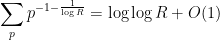
if is large enough. A particular consequence of the growing nature of is that
as this follows from the absolutely convergent nature of the sum  and hence also
  . As a consequence of this, once we “turn off” all the primes less than , any errors in our sieve-theoretic analysis which are quadratic or higher in
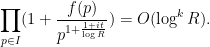
  can be essentially ignored, which will be very convenient for us. In a similar vein, for any fixed -tuple , one has
which allows one to truncate the singular series:

In order to “turn off” all the small primes, we introduce the quantity , defined as the product of all the primes up to (i.e. the primorial of ):

As is going to infinity, is going to infinity also (but as slowly as we please). The idea of the -trick is to search for prime patterns in a single residue class  , which as mentioned earlier will “turn off” all the primes less than in the sieve-theoretic analysis.
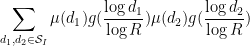
Using (4) and the Chinese remainder theorem, we may thus approximate the singular series as
where  is the Euler totient function of , and
  is the set of residue classes such that all of the shifts
  are coprime to . Note that if consists purely of primes and is sufficiently large, then must lie in one of the residue classes in
  . Thus we can count tuples with all prime by working in each residue class in separately. We conclude that Conjecture 2 is equivalent to the following “-tricked version” in which the singular series is no longer present (or, more precisely, has been replaced by some natural normalisation factors depending on , such as
  ):
):
Conjecture 8 (Prime tuples conjecture, W-tricked quantitative form) Let be a fixed natural number, and let be a fixed admissible -tuple. Assume is a sufficiently slowly growing function of . Then for any residue class in , the number of natural numbers with  such that consists entirely of primes is
  .
.
We will work with similarly -tricked asymptotics in the analysis below.
— 2. Sums of multiplicative functions —
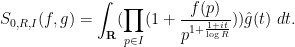
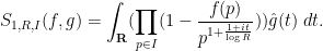
As a result of the sieve-theoretic computations to follow, we will frequently need to estimate sums of the form

and

where  is a multiplicative function, the sieve level
  (also denoted
  in some literature) is a fixed power of (such as
  or
or  ),
),  is the Möbius function,
  is a fixed smooth compactly supported function,
  is a (possibly half-infinite) interval in
  , and
, and  is the set of square-free numbers that are products
  of distinct primes
  in . (Actually, in applications
  won’t quite be smooth, but instead have some high order of differentiability (e.g.
  times continuously differentiable for some
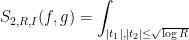
  ), but we can extend the analysis of smooth to sufficiently differentiable by various standard limiting or approximation arguments which we will not dwell on here.) We will also need to control the more complicated variant
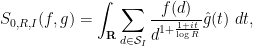
![\displaystyle S_{2,R,I}(f,g_1,g_2) := \sum_{d_1,d_2 \in {\mathcal S}_I} \frac{\mu(d_1) \mu(d_2) f([d_1,d_2])}{[d_1,d_2]} g_1( \frac{\log d_1}{\log R} ) g_2( \frac{\log d_2}{\log R} )](https://s0.wp.com/latex.php?latex=%5Cdisplaystyle+S_%7B2%2CR%2CI%7D%28f%2Cg_1%2Cg_2%29+%3A%3D+%5Csum_%7Bd_1%2Cd_2+%5Cin+%7B%5Cmathcal+S%7D_I%7D+%5Cfrac%7B%5Cmu%28d_1%29+%5Cmu%28d_2%29+f%28%5Bd_1%2Cd_2%5D%29%7D%7B%5Bd_1%2Cd_2%5D%7D+g_1%28+%5Cfrac%7B%5Clog+d_1%7D%7B%5Clog+R%7D+%29+g_2%28+%5Cfrac%7B%5Clog+d_2%7D%7B%5Clog+R%7D+%29&bg=ffffff&fg=000000&s=0&c=20201002)
where  are also smooth compactly supported functions. In practice, the interval will be something like
  ,
,  ,
, ![{[x^\varpi,x^{1/4+\varpi}]}](https://s0.wp.com/latex.php?latex=%7B%5Bx%5E%5Cvarpi%2Cx%5E%7B1%2F4%2B%5Cvarpi%7D%5D%7D&bg=ffffff&fg=000000&s=0&c=20201002) . In particular, thanks to the -trick we will be able to turn off all the primes up to , so that only contains primes larger than , allowing us to take advantage of bounds such as (2).
. In particular, thanks to the -trick we will be able to turn off all the primes up to , so that only contains primes larger than , allowing us to take advantage of bounds such as (2).
Once is restricted to , the quantity  is determined entirely by the values of the multiplicative function
  at primes in :

In applications, will have the size bound
for all  and some fixed positive (note that we allow the implied constants in the
  notation to depend on quantities such as ); we refer to as the dimension of the multiplicative function . Henceforth we assume that has a fixed dimension . We remark that we could unify the treatment of
  and
and  in what follows by allowing multiplicative functions of negative dimension, but we will avoid doing so here. In our applications will be an integer; one could also generalise much of the discussion below to the fractional dimension case, but we will not need to do so here.
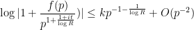
Traditionally the above expressions are handled by complex analysis, starting with Perron’s formula. We will instead take a slightly different Fourier-analytic approach. We perform a Fourier expansion of the smooth compactly supported function  to obtain a representation

for some Schwartz function  ; in particular, is rapidly decreasing. (Strictly speaking, is the Fourier transform of shifted in the complex domain by
  , rather than the true Fourier transform of , but we will ignore this distinction for the purposes of this discussion.) In particular we have

for any . By Fubini’s theorem, we can thus write as
which factorises as
Similarly one has
and

In order to use asymptotics of the Riemann zeta function near the pole  , it is convenient to temporarily truncate the above integrals to the region
  or
or  :
:
Lemma 9 For any fixed  , we have

and

and


Also we have the crude bound

Proof: We begin with the bounds on . From (6) we have
for (which forces  , so there is no issue with the singularity of the logarithm) and thus

Since
we see on taking logarithms that
and thus
The bounds on  then follow from the rapid decrease of . The bounds for and
  are proven similarly.
From (6) and the restriction of to quantities larger than , we see that
and

and


where  is the restricted Euler product
which is well-defined for  at least (and this is the only region of
  for which we will need ).
We now specialise to the model case  , in which case

where 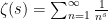 is the Riemann zeta function. Using the basic (and easily proven) asymptotic
  for near

for  , if is sufficiently slowly growing (this can be seen by first working with a fixed large and then using Lemma 7). Note that because of the above truncation, we do not need any deeper bounds on
  than what one can obtain from the simple pole at ; in particular no zero-free regions near the line
  are needed here. (This is ultimately because of the smooth nature of , which is sufficient for the applications in this post; if one wanted rougher cutoff functions here then the situation is closer to that of the prime number theorem, and non-trivial zero-free regions would be required.)
We conclude in the case that


and

and


using the rapid decrease of  , we thus have

and

and


We can rewrite these expressions in terms of instead of . Using the Gamma function identity

and (7) we see that

whilst from differentiating (7) times at the origin (after first dividing by  ) we see that

Combining these two methods, we also see that


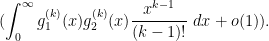
We have thus obtained the following asymptotics:
Proposition 10 (Asymptotics without prime truncation) Suppose that , and that has dimension for some fixed natural number . Then we have

and

and

These asymptotics will suffice for the treatment of the Goldston-Pintz-Yildirim theorem (Theorem 4). For the Motohashi-Pintz-Zhang theorem (Theorem 5) we will also need to deal with truncated intervals , such as  ; we will discuss how to deal with these truncations later.
— 3. The Goldston-Yildirim-Pintz theorem —
We are now ready to state and prove the Goldston-Yildirim-Pintz theorem. We first need to state the Elliott-Halberstam conjecture properly.
Let  be the von Mangoldt function, thus
  equals
  when is equal to a prime or a power of that prime, and equal to zero otherwise. The prime number theorem in arithmetic progressions tells us that

for any fixed arithmetic progression  with
with  coprime to
  . In particular,

where  are the residue classes mod that are coprime to . By invoking the Siegel-Walfisz theorem one can obtain the improvement
for any fixed (though, annoyingly, the implied constant here is only ineffectively bounded with current methods; see this previous post for further discussion).
The above error term is only useful when is fixed (or is of logarithmic size in ). For larger values of , it is very difficult to get good error terms for each separately, unless one assumes powerful hypotheses such as the generalised Riemann hypothesis. However, it is possible to obtain good control on the error term if one averages in . More precisely, for any  , let denote the following assertion:
Conjecture 11 () One has


for all fixed .
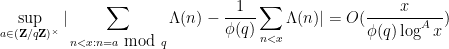
This should be compared with the asymptotic  for some absolute constant
  , as can be deduced for instance from Proposition 10. The Elliott-Halberstam conjecture is the assertion that holds for all . This remains open, but the important Bombieri-Vinogradov theorem establishes for all
  . Remarkably, the threshold
  is also the limit of what one can establish if one directly invokes the generalised Riemann hypothesis, so the Bombieri-Vinogradov theorem is often referred to as an assertion that the generalised Riemann hypothesis (or at least the Siegel-Walfisz theorem) holds “on the average”, which is often good enough for sieve-theoretic purposes.
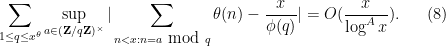
We may replace the von Mangoldt function with the slight variant  , defined to equal when is a prime and zero otherwise. Using this replacement, as well as the prime number theorem (with
 error term), it is not difficult to show that is equivalent to the estimate
Now we establish Theorem 4. Suppose that holds for some fixed  , let be sufficiently large depending on but otherwise fixed, and let be a fixed admissible -tuple. We would like to show that there are infinitely many such that contains at least two primes. We will begin with the -trick, restricting to a residue class with
  (note that is non-empty because is admissible).
The general strategy will be as follows. We will introduce a weight function  that obeys the upper bound

and lower bound

for all  and some fixed
  , where
  is a fixed power of (we will eventually take
  ). (The factors of
  , , and
  on the right-hand side are natural normalisations coming from sieve theory and the reader should not pay too much attention to them.) Informally, (9) says that
  has some normalised density at most
  , and then (10) roughly speaking asserts that relative to the weight ,
  has a probability of at least
  of being prime. If we sum (10) for all
  and then subtract off
  copies of (9), we conclude that
In particular, if we have the crucial inequality

we conclude that

and so  is positive for at least one value of between and
  . This can only occur if contains two or more primes. Thus we must have containing at least two primes for some between and ; sending off to infinity then gives as desired.
It thus suffices to find a weight function obeying the required properties (9), (10) with parameters  obeying the key inequality (11). It is thus of interest to make as large a power of as possible, and to minimise the ratio between and
  . It is in the former task that the Elliott-Halberstam hypothesis will be crucial.
The key is to find a good choice of , and the selection of this weight is arguably the main contribution of Goldston, Pintz, and Yildirim, who use a carefully modified version of the Selberg sieve. Following (a slight modification of) the Goldston-Pintz-Yildirim argument, we will take a weight of the form  , where

where  is a fixed smooth non-negative function supported on
 ![{[-1,1]}](https://s0.wp.com/latex.php?latex=%7B%5B-1%2C1%5D%7D&bg=ffffff&fg=000000&s=0&c=20201002) to be chosen later,
to be chosen later,  , and
, and  is the polynomial
The intuition here is that  is a truncated approximation to a function of the form
for some natural number , which one can check is only non-vanishing when has at most distinct prime factors in . So  is concentrated on those numbers for which already has few prime factors for , which will assist in making the ratio
  as small as possible.
Clearly is non-negative. Now we consider the task of estimating the left-hand side of (9). Expanding out  using (12) and interchanging summations, we can expand this expression as
The constraint  is equivalent to requiring that for each prime dividing
 ![{[d_1,d_2]}](https://s0.wp.com/latex.php?latex=%7B%5Bd_1%2Cd_2%5D%7D&bg=ffffff&fg=000000&s=0&c=20201002) , lies in one of the residue classes
, lies in one of the residue classes  for
for  . By choice of ,
  , so all the
  are distinct, and so we are constraining to lie in one of residue classes modulo for each
 ![{p|[d_1,d_2]}](https://s0.wp.com/latex.php?latex=%7Bp%7C%5Bd_1%2Cd_2%5D%7D&bg=ffffff&fg=000000&s=0&c=20201002) ; together with the constraint
; together with the constraint  and the Chinese remainder theorem, we are thus constraining to
 ![{k_0^{\Omega([d_1,d_2])}}](https://s0.wp.com/latex.php?latex=%7Bk_0%5E%7B%5COmega%28%5Bd_1%2Cd_2%5D%29%7D%7D&bg=ffffff&fg=000000&s=0&c=20201002) residue classes modulo
residue classes modulo ![{W [d_1,d_2]}](https://s0.wp.com/latex.php?latex=%7BW+%5Bd_1%2Cd_2%5D%7D&bg=ffffff&fg=000000&s=0&c=20201002) , where
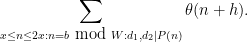
, where ![{\Omega([d_1,d_2])}](https://s0.wp.com/latex.php?latex=%7B%5COmega%28%5Bd_1%2Cd_2%5D%29%7D&bg=ffffff&fg=000000&s=0&c=20201002) is the number of prime factors of . We thus have
is the number of prime factors of . We thus have
![\displaystyle \sum_{x \leq n \leq 2x: n = b \hbox{ mod } W: d_1,d_2 | P(n)} 1 = k_0^{\Omega([d_1,d_2])} \frac{x}{W[d_1,d_2]} + O( k_0^{\Omega([d_1,d_2])} ).](https://s0.wp.com/latex.php?latex=%5Cdisplaystyle+%5Csum_%7Bx+%5Cleq+n+%5Cleq+2x%3A+n+%3D+b+%5Chbox%7B+mod+%7D+W%3A+d_1%2Cd_2+%7C+P%28n%29%7D+1+%3D+k_0%5E%7B%5COmega%28%5Bd_1%2Cd_2%5D%29%7D+%5Cfrac%7Bx%7D%7BW%5Bd_1%2Cd_2%5D%7D+%2B+O%28+k_0%5E%7B%5COmega%28%5Bd_1%2Cd_2%5D%29%7D+%29.&bg=ffffff&fg=000000&s=0&c=20201002)
Note from the support of that  may be constrained to be at most , so that
  is at most
  . We can thus express the left-hand side of (9) as the main term
![\displaystyle \sum_{d_1,d_2 \in {\mathcal S}_I} \mu(d_1) g(\frac{\log d_1}{\log R}) \mu(d_2) g(\frac{\log d_2}{\log R}) k_0^{\Omega([d_1,d_2])} \frac{x}{W[d_1,d_2]}](https://s0.wp.com/latex.php?latex=%5Cdisplaystyle+%5Csum_%7Bd_1%2Cd_2+%5Cin+%7B%5Cmathcal+S%7D_I%7D+%5Cmu%28d_1%29+g%28%5Cfrac%7B%5Clog+d_1%7D%7B%5Clog+R%7D%29+%5Cmu%28d_2%29+g%28%5Cfrac%7B%5Clog+d_2%7D%7B%5Clog+R%7D%29+k_0%5E%7B%5COmega%28%5Bd_1%2Cd_2%5D%29%7D+%5Cfrac%7Bx%7D%7BW%5Bd_1%2Cd_2%5D%7D+&bg=ffffff&fg=000000&s=0&c=20201002)
plus an error

By Proposition 10, the error term is  . So if we set

then the error term will certainly give a negligible contribution to (9) with plenty of room to spare. (But when we come to the more difficult sum (10), we will have much less room – only a superlogarithmic amount of room, in fact.) To show (9), it thus suffices to show that
![\displaystyle \sum_{d_1,d_2 \in {\mathcal S}_I} \mu(d_1) g(\frac{\log d_1}{\log R}) \mu(d_2) g(\frac{\log d_2}{\log R}) \frac{k_0^{\Omega([d_1,d_2])}}{[d_1,d_2]}](https://s0.wp.com/latex.php?latex=%5Cdisplaystyle+%5Csum_%7Bd_1%2Cd_2+%5Cin+%7B%5Cmathcal+S%7D_I%7D+%5Cmu%28d_1%29+g%28%5Cfrac%7B%5Clog+d_1%7D%7B%5Clog+R%7D%29+%5Cmu%28d_2%29+g%28%5Cfrac%7B%5Clog+d_2%7D%7B%5Clog+R%7D%29+%5Cfrac%7Bk_0%5E%7B%5COmega%28%5Bd_1%2Cd_2%5D%29%7D%7D%7B%5Bd_1%2Cd_2%5D%7D+&bg=ffffff&fg=000000&s=0&c=20201002)

But by Proposition 10 (applied to the -dimensional multiplicative function ) and the support of , this bound holds with equal to the quantity
Now we turn to (10). Fix . Repeating the arguments for (9), we may expand the left-hand side of (10) as
Now we consider the inner sum
As discussed earlier, the conditions and split into residue classes ![{n = a \hbox{ mod } W [d_1,d_2]}](https://s0.wp.com/latex.php?latex=%7Bn+%3D+a+%5Chbox%7B+mod+%7D+W+%5Bd_1%2Cd_2%5D%7D&bg=ffffff&fg=000000&s=0&c=20201002) . However, if
. However, if  for one of the primes dividing , then
  must vanish (since
  is much less than ). So there are actually only
 ![{(k_0-1)^{\Omega([d_1,d_2])}}](https://s0.wp.com/latex.php?latex=%7B%28k_0-1%29%5E%7B%5COmega%28%5Bd_1%2Cd_2%5D%29%7D%7D&bg=ffffff&fg=000000&s=0&c=20201002) residue classes
residue classes ![{a \hbox{ mod } W[d_1,d_2]}](https://s0.wp.com/latex.php?latex=%7Ba+%5Chbox%7B+mod+%7D+W%5Bd_1%2Cd_2%5D%7D&bg=ffffff&fg=000000&s=0&c=20201002) for which
for which  is coprime to
 ![{W[d_1,d_2]}](https://s0.wp.com/latex.php?latex=%7BW%5Bd_1%2Cd_2%5D%7D&bg=ffffff&fg=000000&s=0&c=20201002) . We thus have
. We thus have
![\displaystyle \sum_{x \leq n \leq 2x: n = a \hbox{ mod } W[d_1,d_2]} \theta(n+h) = (k_0-1)^{\Omega([d_1,d_2])} \frac{x}{\phi(W[d_1,d_2])}](https://s0.wp.com/latex.php?latex=%5Cdisplaystyle+%5Csum_%7Bx+%5Cleq+n+%5Cleq+2x%3A+n+%3D+a+%5Chbox%7B+mod+%7D+W%5Bd_1%2Cd_2%5D%7D+%5Ctheta%28n%2Bh%29+%3D+%28k_0-1%29%5E%7B%5COmega%28%5Bd_1%2Cd_2%5D%29%7D+%5Cfrac%7Bx%7D%7B%5Cphi%28W%5Bd_1%2Cd_2%5D%29%7D+&bg=ffffff&fg=000000&s=0&c=20201002)
![\displaystyle + O( (k_0-1)^{\Omega([d_1,d_2])} E(x; W[d_1,d_2]) )](https://s0.wp.com/latex.php?latex=%5Cdisplaystyle+%2B+O%28+%28k_0-1%29%5E%7B%5COmega%28%5Bd_1%2Cd_2%5D%29%7D+E%28x%3B+W%5Bd_1%2Cd_2%5D%29+%29&bg=ffffff&fg=000000&s=0&c=20201002)
where  denotes the quantity
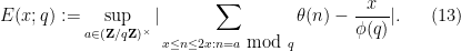
Remark 1 There is an inefficiency here; the supremum in (13) is over all primitive residue classes , but actually one only needs to take the supremum over the  residue classes for which
  , where
  . This inefficiency is not exploitable if we insist on using the Elliott-Halberstam conjecture as the starting hypothesis, but will be used in the arguments of the next section in which a more lightweight hypothesis is utilised.
The left-hand side of (10) is thus equal to the main term
![\displaystyle \sum_{d_1,d_2 \in {\mathcal S}_I} \mu(d_1) g(\frac{\log d_1}{\log R}) \mu(d_2) g(\frac{\log d_2}{\log R}) (k_0-1)^{\Omega([d_1,d_2])} \frac{x}{\phi(W[d_1,d_2])}](https://s0.wp.com/latex.php?latex=%5Cdisplaystyle+%5Csum_%7Bd_1%2Cd_2+%5Cin+%7B%5Cmathcal+S%7D_I%7D+%5Cmu%28d_1%29+g%28%5Cfrac%7B%5Clog+d_1%7D%7B%5Clog+R%7D%29+%5Cmu%28d_2%29+g%28%5Cfrac%7B%5Clog+d_2%7D%7B%5Clog+R%7D%29+%28k_0-1%29%5E%7B%5COmega%28%5Bd_1%2Cd_2%5D%29%7D+%5Cfrac%7Bx%7D%7B%5Cphi%28W%5Bd_1%2Cd_2%5D%29%7D&bg=ffffff&fg=000000&s=0&c=20201002)
plus an error term
![\displaystyle O( \sum_{d_1,d_2 \in {\mathcal S}_I} g(\frac{\log d_1}{\log R}) g(\frac{\log d_2}{\log R}) (k_0-1)^{\Omega([d_1,d_2])} E(x; W[d_1,d_2]) ).](https://s0.wp.com/latex.php?latex=%5Cdisplaystyle+O%28+%5Csum_%7Bd_1%2Cd_2+%5Cin+%7B%5Cmathcal+S%7D_I%7D+g%28%5Cfrac%7B%5Clog+d_1%7D%7B%5Clog+R%7D%29+g%28%5Cfrac%7B%5Clog+d_2%7D%7B%5Clog+R%7D%29+%28k_0-1%29%5E%7B%5COmega%28%5Bd_1%2Cd_2%5D%29%7D+E%28x%3B+W%5Bd_1%2Cd_2%5D%29+%29.&bg=ffffff&fg=000000&s=0&c=20201002)
We first deal with the error term. Since is in and is bounded by on the support of this function, and each  has
has  representations of the form
 ![{d = [d_1,d_2]}](https://s0.wp.com/latex.php?latex=%7Bd+%3D+%5Bd_1%2Cd_2%5D%7D&bg=ffffff&fg=000000&s=0&c=20201002) , we can bound this expression by
, we can bound this expression by

Note that we are assuming to be a fixed smooth compactly supported function and so it has magnitude . On the other hand, from Proposition 10 and the trivial bound  we have

while from (8) (and here we crucially use the choice of ) one easily verifies that
for any fixed  . By the Cauchy-Schwarz inequality we see that the error term to (10) is negligible (assuming sufficiently slowly growing of course). Meanwhile, the main term can be rewritten as
![\displaystyle \frac{x}{\phi(W)} \sum_{d_1,d_2 \in {\mathcal S}_I} \mu(d_1) g(\frac{\log d_1}{\log R}) \mu(d_2) g(\frac{\log d_2}{\log R}) \frac{f([d_1,d_2])}{[d_1,d_2]}](https://s0.wp.com/latex.php?latex=%5Cdisplaystyle+%5Cfrac%7Bx%7D%7B%5Cphi%28W%29%7D+%5Csum_%7Bd_1%2Cd_2+%5Cin+%7B%5Cmathcal+S%7D_I%7D+%5Cmu%28d_1%29+g%28%5Cfrac%7B%5Clog+d_1%7D%7B%5Clog+R%7D%29+%5Cmu%28d_2%29+g%28%5Cfrac%7B%5Clog+d_2%7D%7B%5Clog+R%7D%29+%5Cfrac%7Bf%28%5Bd_1%2Cd_2%5D%29%7D%7B%5Bd_1%2Cd_2%5D%7D&bg=ffffff&fg=000000&s=0&c=20201002)
where is the  -dimensional multiplicative function
Applying Proposition 10, we obtain (10) with
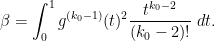
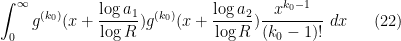
To obtain the crucial inequality (11), we thus need to locate a fixed smooth non-negative function supported on obeying the inequality

In principle one can use calculus of variations to optimise the choice of here (it will be the ground state of a certain one-dimensional Schrödinger operator), but one can already get a fairly good result here by a specific choice of that is amenable for computations, namely a polynomial of the form 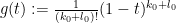 for
for ![{t \in [0,1]}](https://s0.wp.com/latex.php?latex=%7Bt+%5Cin+%5B0%2C1%5D%7D&bg=ffffff&fg=000000&s=0&c=20201002) and some integer , with vanishing for
and some integer , with vanishing for  and smoothly truncated to somehow at negative values of
  . Strictly speaking, this is not admissible here because it is not infinitely smooth at , being only times continuously differentiable instead, but one can regularise this function to be smooth without significantly affecting either side of (14), so we will go ahead and test (14) with this function and leave the regularisation details to the reader. The inequality then becomes (after cancelling some factors)

Using the Beta function identity
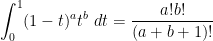
we have

and

and the preceding equation now becomes
which simplifies to

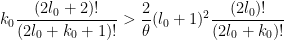
Actually, the same inequality is also applicable when  is real instead of integer, using Gamma functions in place of factorials; we leave the details to the interested reader. We can then optimise in by setting
  , arriving at the inequality
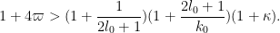
But as long as  , this inequality is satisfiable for any larger than
  . This concludes the proof of Theorem 4.
Remark 2 One can obtain slightly better dependencies of in terms of by using more general functions for than the monomials  , for instance one can take linear combinations of such functions. See the paper of Goldston, Pintz, and Yildirim for details. Unfortunately, as noted in this survey of Soundararajan, one has the general inequality

which defeats any attempt to directly use this method using only the Bombieri-Vinogradov result that holds for all  . We show (17) in the case when is large. Write
  , then (17) simplifies to

The right-hand side simplifies after some integration by parts to

Subtracting off  from both sides, one is left with

From the fundamental theorem of calculus and Cauchy-Schwarz, one has the bound
Using this bound for  close to and dominating
  by
by  for far from , we obtain the claim (at least if is large enough). There is some slack in this argument; it would be of interest to calculate exactly what the best constants are in (17), so that one can obtain the optimal relationship between and .
To get around this obstruction (17) in the unconditional setting when one only has for , Goldston, Pintz, and Yildirim also considered sums of the form  in which
  was now outside (but close to) . While the bounds here were significantly inferior to those in (10), they were still sufficient to prove a variant of the inequality (11) to get reasonably small gaps between primes.
— 4. The Motohashi-Pintz-Zhang theorem —
We now modify the above argument to give Theorem 5. Our treatment here is different from that of Zhang in that it employs the method of Buchstab iteration; a related argument also appears in the paper of Motohashi and Pintz. This arrangement of the argument leads to a more efficient dependence of on  than in the paper of Zhang. (The argument of Motohashi and Pintz is a bit more complicated and uses a slightly different formulation of the base conjecture , but the final bounds are similar to those given here, albeit with non-explicit constants in the notation.)
The main idea here is to truncate the interval of relevant primes from  to
to  for some small . Somewhat remarkably, it turns out that this apparently severe truncation does not affect the sums (9), (10) here as long as
  is large (which is going to be the case in practice, with being comparable to
  ). The intuition is that was already concentrated on those for which had about
  factors, and it is too “expensive” for one of these factors to as large as
  or more, as it forces many of the other factors to be smaller than they “want” to be. The advantage of truncating the set of primes this way is that the version of the Elliott-Halberstam conjecture needed also acquires the same truncation, which gives that version a certain “well-factored” form (in the spirit of the work of Bombieri, Fouvry, Friedlander, and Iwaniec) which is essential in being able to establish that conjecture unconditionally for some suitably small .
To make this more precise, we first formalise the conjecture for mentioned earlier.
Conjecture 12 () Let be a fixed -tuple (not necessarily admissible) for some fixed  , and let be a primitive residue class. Then

for any fixed , where  and
and  is the quantity


and
This is the -tricked formulation of the conjecture as (implicitly) stated in Zhang’s paper, which did not have the restriction present (and with the interval enlarged from to  , and
, and  was required to be admissible). However the two formulations are morally equivalent (and Zhang’s arguments establish Theorem 6 with as stated). From the prime number theorem in arithmetic progressions (with
  error term) together with Proposition 10 we observe that we may replace (18) here by the slight variant


without affecting the truth of .
It is also not difficult to deduce from ![{EH[1/2 + 2 \varpi]}](https://s0.wp.com/latex.php?latex=%7BEH%5B1%2F2+%2B+2+%5Cvarpi%5D%7D&bg=ffffff&fg=000000&s=0&c=20201002) after using a Cauchy-Schwarz argument to dispose of the
after using a Cauchy-Schwarz argument to dispose of the  residue classes in the above sum (cf. the treatment of the error term in (10) in the previous section); we leave the details to the interested reader. Note however that whilst
 ![{EH[1/2+2\varpi]}](https://s0.wp.com/latex.php?latex=%7BEH%5B1%2F2%2B2%5Cvarpi%5D%7D&bg=ffffff&fg=000000&s=0&c=20201002) demands control over all primitive residue classes in a given modulus , the conjecture only requires control of a much smaller number of residue classes (roughly polylogarithmic in number, on average). Thus is simpler than , though it is still far from trivial.
demands control over all primitive residue classes in a given modulus , the conjecture only requires control of a much smaller number of residue classes (roughly polylogarithmic in number, on average). Thus is simpler than , though it is still far from trivial.
We now begin the proof of Theorem 5. Let be such that holds, and let be a sufficiently large quantity depending on but which is otherwise fixed. As before, it suffices to locate a non-negative sieve weight that obeys the estimates (9), (10) for parameters that obey the key inequality (11), and with smooth and supported on . The choice of weight is almost the same as before; it is also given as a square with given by (12), but now the interval is truncated to instead of  . Also, in this argument we take

We now establish (9). By repeating the previous arguments, the left-hand side of (9) is equal to a main term
![\displaystyle \sum_{d_1,d_2 \in {\mathcal S}_I} \mu(d_1) g(\frac{\log d_1}{\log R}) \mu(d_2) g(\frac{\log d_2}{\log R}) k_0^{\Omega([d_1,d_2])} \frac{x}{W[d_1,d_2]} \ \ \ \ \ (20)](https://s0.wp.com/latex.php?latex=%5Cdisplaystyle+%5Csum_%7Bd_1%2Cd_2+%5Cin+%7B%5Cmathcal+S%7D_I%7D+%5Cmu%28d_1%29+g%28%5Cfrac%7B%5Clog+d_1%7D%7B%5Clog+R%7D%29+%5Cmu%28d_2%29+g%28%5Cfrac%7B%5Clog+d_2%7D%7B%5Clog+R%7D%29+k_0%5E%7B%5COmega%28%5Bd_1%2Cd_2%5D%29%7D+%5Cfrac%7Bx%7D%7BW%5Bd_1%2Cd_2%5D%7D+%5C+%5C+%5C+%5C+%5C+%2820%29&bg=ffffff&fg=000000&s=0&c=20201002)
plus an error term which continues to be acceptable (indeed, the error term is slightly smaller than in the previous case due to the truncated nature of ). At this point in the previous section we applied Proposition 10, but that proposition was only available for the untruncated interval  instead of the truncated interval
  . One could try to adapt the proof of that proposition to the truncated case, but then one is faced with the problem of controlling the truncated zeta function . While one can eventually get some reasonable asymptotics for this function, it seems to be more efficient to eschew Fourier analysis and work entirely in “physical space” by the following partial Möbius inversion argument. Write
  , thus
  . Observe that for any
  , the quantity
  equals when lies in and vanishes otherwise. Hence, for any function
  of
of  and
and  supported on squarefree numbers we have the partial Mobius inversion formula

and so the main term (20) can be expressed as

![\displaystyle k_0^{\Omega([a_1d_1,a_2d_2])} \frac{x}{W [a_1d_1,a_2d_2]}.](https://s0.wp.com/latex.php?latex=%5Cdisplaystyle+k_0%5E%7B%5COmega%28%5Ba_1d_1%2Ca_2d_2%5D%29%7D+%5Cfrac%7Bx%7D%7BW+%5Ba_1d_1%2Ca_2d_2%5D%7D.&bg=ffffff&fg=000000&s=0&c=20201002)
We first dispose of the contribution to (21) when  share a common prime factor
  for some
  . For any fixed
  , we can bound this contribution by
![\displaystyle \ll \frac{x}{W} \sum_{p_* \in J} \sum_{a_1,a_2 \in {\mathcal S}_J} \sum_{d_1,d_2 \in {\mathcal S}_{I \cup J}} 1_{p^2_*|a_id_j} (a_1 d_1 a_2 d_2)^{-1/\log R} \frac{k_0^{\Omega([a_1d_1,a_2d_2])}}{[a_1d_1,a_2d_2]}.](https://s0.wp.com/latex.php?latex=%5Cdisplaystyle+%5Cll+%5Cfrac%7Bx%7D%7BW%7D+%5Csum_%7Bp_%2A+%5Cin+J%7D+%5Csum_%7Ba_1%2Ca_2+%5Cin+%7B%5Cmathcal+S%7D_J%7D+%5Csum_%7Bd_1%2Cd_2+%5Cin+%7B%5Cmathcal+S%7D_%7BI+%5Ccup+J%7D%7D+1_%7Bp%5E2_%2A%7Ca_id_j%7D+%28a_1+d_1+a_2+d_2%29%5E%7B-1%2F%5Clog+R%7D+%5Cfrac%7Bk_0%5E%7B%5COmega%28%5Ba_1d_1%2Ca_2d_2%5D%29%7D%7D%7B%5Ba_1d_1%2Ca_2d_2%5D%7D.&bg=ffffff&fg=000000&s=0&c=20201002)
Factorising the inner two sums as an Euler product, this becomes
[UPDATE: The above argument is not quite correct; a corrected (and improved) version is given at this newer post.] The product is  by e.g. Mertens’ theorem, while
  . So the contribution of this case is negligible.
If do not share a common factor for any , then we can factor ![{[a_1d_1,a_2d_2]}](https://s0.wp.com/latex.php?latex=%7B%5Ba_1d_1%2Ca_2d_2%5D%7D&bg=ffffff&fg=000000&s=0&c=20201002) as
as ![{[a_1,a_2][d_1,d_2]}](https://s0.wp.com/latex.php?latex=%7B%5Ba_1%2Ca_2%5D%5Bd_1%2Cd_2%5D%7D&bg=ffffff&fg=000000&s=0&c=20201002) . Rearranging this portion of (21) and then reinserting the case when have a common factor for some , we may write (21) up to negligible errors as
. Rearranging this portion of (21) and then reinserting the case when have a common factor for some , we may write (21) up to negligible errors as
![\displaystyle \frac{x}{W} \sum_{a_1, a_2 \in {\mathcal S}_J} \frac{k_0^{\Omega([a_1,a_2])}}{[a_1,a_2]} \sum_{d_1,d_2 \in {\mathcal S}_{I \cup J}} \mu(d_1) g(\frac{\log d_1}{\log R} + \frac{\log a_1}{\log R})](https://s0.wp.com/latex.php?latex=%5Cdisplaystyle+%5Cfrac%7Bx%7D%7BW%7D+%5Csum_%7Ba_1%2C+a_2+%5Cin+%7B%5Cmathcal+S%7D_J%7D+%5Cfrac%7Bk_0%5E%7B%5COmega%28%5Ba_1%2Ca_2%5D%29%7D%7D%7B%5Ba_1%2Ca_2%5D%7D+%5Csum_%7Bd_1%2Cd_2+%5Cin+%7B%5Cmathcal+S%7D_%7BI+%5Ccup+J%7D%7D+%5Cmu%28d_1%29+g%28%5Cfrac%7B%5Clog+d_1%7D%7B%5Clog+R%7D+%2B+%5Cfrac%7B%5Clog+a_1%7D%7B%5Clog+R%7D%29+&bg=ffffff&fg=000000&s=0&c=20201002)
![\displaystyle \mu(d_2) g(\frac{\log d_2}{\log R} + \frac{\log a_2}{\log R}) \frac{k_0^{\Omega([d_1,d_2])}}{[d_1,d_2]}.](https://s0.wp.com/latex.php?latex=%5Cdisplaystyle+%5Cmu%28d_2%29+g%28%5Cfrac%7B%5Clog+d_2%7D%7B%5Clog+R%7D+%2B+%5Cfrac%7B%5Clog+a_2%7D%7B%5Clog+R%7D%29+%5Cfrac%7Bk_0%5E%7B%5COmega%28%5Bd_1%2Cd_2%5D%29%7D%7D%7B%5Bd_1%2Cd_2%5D%7D.&bg=ffffff&fg=000000&s=0&c=20201002)
Note that we can restrict  to be at most as otherwise the factors vanish. The inner sum
![\displaystyle \sum_{d_1,d_2 \in {\mathcal S}_{I \cup J}} \mu(d_1) g(\frac{\log d_1}{\log R} + \frac{\log a_1}{\log R}) \mu(d_2) g(\frac{\log d_2}{\log R} + \frac{\log a_2}{\log R}) \frac{k_0^{\Omega([d_1,d_2])}}{[d_1,d_2]}](https://s0.wp.com/latex.php?latex=%5Cdisplaystyle+%5Csum_%7Bd_1%2Cd_2+%5Cin+%7B%5Cmathcal+S%7D_%7BI+%5Ccup+J%7D%7D+%5Cmu%28d_1%29+g%28%5Cfrac%7B%5Clog+d_1%7D%7B%5Clog+R%7D+%2B+%5Cfrac%7B%5Clog+a_1%7D%7B%5Clog+R%7D%29+%5Cmu%28d_2%29+g%28%5Cfrac%7B%5Clog+d_2%7D%7B%5Clog+R%7D+%2B+%5Cfrac%7B%5Clog+a_2%7D%7B%5Clog+R%7D%29+%5Cfrac%7Bk_0%5E%7B%5COmega%28%5Bd_1%2Cd_2%5D%29%7D%7D%7B%5Bd_1%2Cd_2%5D%7D+&bg=ffffff&fg=000000&s=0&c=20201002)
is now of the form that can be treated by Proposition 10, and takes the form


Here we make the technical remark that the translates of by shifts between  and are uniformly controlled in smooth norms, which means that the error here is uniform in the choices of
  .
.
Let us first deal with the contribution of the error term. This is bounded by
![\displaystyle o( \frac{x}{W} (\frac{\phi(W)}{W} \log R)^{-k_0} \sum_{a_1,a_2 \in {\mathcal S}_{(x^\varpi, R]}} \frac{k_0^{\Omega([a_1,a_2])}}{[a_1,a_2]} ).](https://s0.wp.com/latex.php?latex=%5Cdisplaystyle+o%28+%5Cfrac%7Bx%7D%7BW%7D+%28%5Cfrac%7B%5Cphi%28W%29%7D%7BW%7D+%5Clog+R%29%5E%7B-k_0%7D+%5Csum_%7Ba_1%2Ca_2+%5Cin+%7B%5Cmathcal+S%7D_%7B%28x%5E%5Cvarpi%2C+R%5D%7D%7D+%5Cfrac%7Bk_0%5E%7B%5COmega%28%5Ba_1%2Ca_2%5D%29%7D%7D%7B%5Ba_1%2Ca_2%5D%7D+%29.&bg=ffffff&fg=000000&s=0&c=20201002)
The inner sum factorises as
which by Mertens’ theorem is (albeit with a rather large implied constant!), so this error is negligible for the purposes of (9). Indeed, (9) is now reduced to the inequality
![\displaystyle \sum_{a_1,a_2 \in {\mathcal S}_J} \frac{k_0^{\Omega([a_1,a_2])}}{[a_1,a_2]}](https://s0.wp.com/latex.php?latex=%5Cdisplaystyle+%5Csum_%7Ba_1%2Ca_2+%5Cin+%7B%5Cmathcal+S%7D_J%7D+%5Cfrac%7Bk_0%5E%7B%5COmega%28%5Ba_1%2Ca_2%5D%29%7D%7D%7B%5Ba_1%2Ca_2%5D%7D+&bg=ffffff&fg=000000&s=0&c=20201002)

Note that the factor  increases very rapidly with when is large, which basically means that any non-trivial shift of the
  factors to the left by
  or
or  will cause the integral in (22) to decrease dramatically. Since all the in
  are either equal to or bounded below by , this will cause the
  term to dominate in the regime when is large (or more precisely
  ), which is the case in applications.
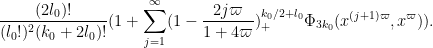
At this point, in order to perform the computations cleanly, we will mimic the arguments from the previous section and take the explicit choice
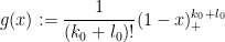
for some integer and  (and some smooth continuation to for negative , and so
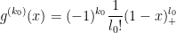
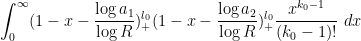
for positive . (Again, this function is not quite smooth at , but this issue can be dealt with by an infinitesimal regularisation argument which we omit here.) The left-hand side of (22) now becomes
![\displaystyle \frac{1}{(l_0!)^2} \sum_{a_1,a_2 \in {\mathcal S}_J} \frac{k_0^{\Omega([a_1,a_2])}}{[a_1,a_2]} \int_0^\infty (1-x-\frac{\log a_1}{\log R})_+^{l_0} (1-x-\frac{\log a_2}{\log R})_+^{l_0}](https://s0.wp.com/latex.php?latex=%5Cdisplaystyle+%5Cfrac%7B1%7D%7B%28l_0%21%29%5E2%7D+%5Csum_%7Ba_1%2Ca_2+%5Cin+%7B%5Cmathcal+S%7D_J%7D+%5Cfrac%7Bk_0%5E%7B%5COmega%28%5Ba_1%2Ca_2%5D%29%7D%7D%7B%5Ba_1%2Ca_2%5D%7D+%5Cint_0%5E%5Cinfty+%281-x-%5Cfrac%7B%5Clog+a_1%7D%7B%5Clog+R%7D%29_%2B%5E%7Bl_0%7D+%281-x-%5Cfrac%7B%5Clog+a_2%7D%7B%5Clog+R%7D%29_%2B%5E%7Bl_0%7D+&bg=ffffff&fg=000000&s=0&c=20201002)

The integral here is a little bit more complicated than a beta integral. To estimate it, we use the beta function identity to observe that

and

and hence by Cauchy-Schwarz
This Cauchy-Schwarz step is a bit wasteful when are far apart, but this does seems to only lead to a minor loss of efficiency in the estimates. We have thus bounded the left-hand side of (22) by
![\displaystyle \frac{(2l_0)!}{(l_0!)^2 (k_0+2l_0)!} \sum_{a_1,a_2 \in {\mathcal S}_J} \frac{k_0^{\Omega([a_1,a_2])}}{[a_1,a_2]}](https://s0.wp.com/latex.php?latex=%5Cdisplaystyle+%5Cfrac%7B%282l_0%29%21%7D%7B%28l_0%21%29%5E2+%28k_0%2B2l_0%29%21%7D+%5Csum_%7Ba_1%2Ca_2+%5Cin+%7B%5Cmathcal+S%7D_J%7D+%5Cfrac%7Bk_0%5E%7B%5COmega%28%5Ba_1%2Ca_2%5D%29%7D%7D%7B%5Ba_1%2Ca_2%5D%7D+&bg=ffffff&fg=000000&s=0&c=20201002)

It is now convenient to collapse the double summation to a single summation. We may bound
![\displaystyle (1 - \frac{\log a_1}{\log R})_+^{k_0/2+l_0} (1 - \frac{\log a_2}{\log R})_+^{k_0/2+l_0} \leq (1 - \frac{\log [a_1,a_2]}{\log R^2})_+^{k_0/2+l_0}](https://s0.wp.com/latex.php?latex=%5Cdisplaystyle+%281+-+%5Cfrac%7B%5Clog+a_1%7D%7B%5Clog+R%7D%29_%2B%5E%7Bk_0%2F2%2Bl_0%7D+%281+-+%5Cfrac%7B%5Clog+a_2%7D%7B%5Clog+R%7D%29_%2B%5E%7Bk_0%2F2%2Bl_0%7D+%5Cleq+%281+-+%5Cfrac%7B%5Clog+%5Ba_1%2Ca_2%5D%7D%7B%5Clog+R%5E2%7D%29_%2B%5E%7Bk_0%2F2%2Bl_0%7D+&bg=ffffff&fg=000000&s=0&c=20201002)
(since ![{\frac{\log [a_1,a_2]}{\log R^2}}](https://s0.wp.com/latex.php?latex=%7B%5Cfrac%7B%5Clog+%5Ba_1%2Ca_2%5D%7D%7B%5Clog+R%5E2%7D%7D&bg=ffffff&fg=000000&s=0&c=20201002) is less than the greater of and ) and observe that each
is less than the greater of and ) and observe that each  has
has  representations of the form
 ![{a = [a_1,a_2]}](https://s0.wp.com/latex.php?latex=%7Ba+%3D+%5Ba_1%2Ca_2%5D%7D&bg=ffffff&fg=000000&s=0&c=20201002) , so we may now bound the left-hand side of (22) by
, so we may now bound the left-hand side of (22) by
Note that an element of  is either equal to , or lies in the interval
  for some natural number
  . In the latter case, we have

In particular, this expression vanishes if  . We can thus bound the left-hand side of (22) by
If we introduce the quantity
then we have thus bounded the left-hand side of (22) by
We observe that
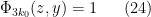
when  , while in general we have the Buchstab identity

as can be seen by isolating the smallest prime  in all the terms in (23) with
  . (This inequality is very close to being an identity, the only loss coming from the possibility of the prime factor being repeated in a term associated to
  .) We can iterate this identity to obtain the following conclusion:
Lemma 13 For any , we have
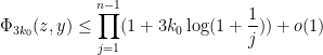
whenever  and
and  for some fixed
  , with the error term being uniform in the choice of
  .
.
Proof: Write  . We prove the bound
  by strong induction on . The case
  follows from (24). Now suppose that
  and that the claim has already been proven for smaller . Let and
  . Note that
  whenever
  . We thus have from (25) and the induction hypothesis that

applying Mertens’ theorem (or the prime number theorem) we have
and the claim follows from the telescoping identity
Applying this inequality, we have established (22) with
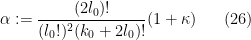
where

We remark that as a first approximation we have
and
so in the regime ,  is roughly
  , which will be negligible for the parameter ranges of
  of interest. Thus the in this argument is quite close to the from (15) in practice.
Now we turn to (10). Fix . As in the previous section, we can bound the left-hand side of (10) as the sum of the main term
plus an error term
![\displaystyle O( \sum_{d_1,d_2 \in {\mathcal S}_I} g(\frac{\log d_1}{\log R}) g(\frac{\log d_2}{\log R}) (k_0-1)^{\Omega([d_1,d_2])} E'(x; [d_1,d_2]) )](https://s0.wp.com/latex.php?latex=%5Cdisplaystyle+O%28+%5Csum_%7Bd_1%2Cd_2+%5Cin+%7B%5Cmathcal+S%7D_I%7D+g%28%5Cfrac%7B%5Clog+d_1%7D%7B%5Clog+R%7D%29+g%28%5Cfrac%7B%5Clog+d_2%7D%7B%5Clog+R%7D%29+%28k_0-1%29%5E%7B%5COmega%28%5Bd_1%2Cd_2%5D%29%7D+E%27%28x%3B+%5Bd_1%2Cd_2%5D%29+%29&bg=ffffff&fg=000000&s=0&c=20201002)
where  is the quantity
 is the polynomial
  , and
, and  was defined in (19). Using the hypothesis and Cauchy-Schwarz as in the previous section we see that the error term is negligible for the purposes of establishing (10). As for the main term, the same argument used to reduce (9) to (22) shows that (10) reduces to
![\displaystyle \sum_{a_1,a_2 \in {\mathcal S}_J} \frac{(k_0-1)^{\Omega([a_1,a_2])}}{\phi([a_1,a_2])} \int_0^\infty g^{(k_0-1)}(x + \frac{\log a_1}{\log R}) g^{(k_0-1)}(x + \frac{\log a_2}{\log R}) \frac{x^{k_0-2}}{(k_0-2)!}\ dx](https://s0.wp.com/latex.php?latex=%5Cdisplaystyle+%5Csum_%7Ba_1%2Ca_2+%5Cin+%7B%5Cmathcal+S%7D_J%7D+%5Cfrac%7B%28k_0-1%29%5E%7B%5COmega%28%5Ba_1%2Ca_2%5D%29%7D%7D%7B%5Cphi%28%5Ba_1%2Ca_2%5D%29%7D+%5Cint_0%5E%5Cinfty+g%5E%7B%28k_0-1%29%7D%28x+%2B+%5Cfrac%7B%5Clog+a_1%7D%7B%5Clog+R%7D%29+g%5E%7B%28k_0-1%29%7D%28x+%2B+%5Cfrac%7B%5Clog+a_2%7D%7B%5Clog+R%7D%29+%5Cfrac%7Bx%5E%7Bk_0-2%7D%7D%7B%28k_0-2%29%21%7D%5C+dx+&bg=ffffff&fg=000000&s=0&c=20201002)

Here, we can do something a bit crude; with our choice of , the integrand is non-negative, so we can simply discard all but the term and reduce to
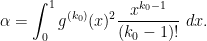
(The intuition here is that by refusing to sieve using primes larger than , we have enlarged the sieve , which makes the upper bound (9) more difficult but the lower bound (10) actually becomes easier.) So we can take the same choice (16) of as in the previous section:

Inserting this and (26) into (11) and simplifying, we see that we can obtain once we can verify the inequality
As before, can be taken to be non-integer if desired. Setting to be slightly larger than  we obtain Theorem 5.
— 5. Using optimal values of (NEW, June 5, 2013) —
We can do better than given above by using an optimal value of . The following result was obtained recently by Farkas, Pintz, and Revesz, and independently worked out by commenters on this blog:
Theorem 14 (Optimal GPY weight) Let  be an integer. Then the ratio

where ![{f: [0,1] \rightarrow {\bf R}}](https://s0.wp.com/latex.php?latex=%7Bf%3A+%5B0%2C1%5D+%5Crightarrow+%7B%5Cbf+R%7D%7D&bg=ffffff&fg=000000&s=0&c=20201002) is a smooth function with
is a smooth function with  that is not identically vanishing, has a minimal value of

where  is the first zero of the Bessel function
  . Furthermore, this minimum is attained if (and only if) is a scalar multiple of the function

Proof: The function , by definition, obeys the Bessel differential equation

and also vanishes to order  at the origin. From this and routine computations it is easy to see that
  is smooth, strictly positive on
  , and obeys the differential equation
If we write  , which is well-defined away from since is non-vanishing on , then
  obeys the Ricatti-type equation

Now consider the quadratic form

for smooth functions with . A calculation using (29) and integration by parts shows that

and so  , giving the first claim; the second claim follows by noting that
  vanishes if and only if is a scalar multiple of . (Note that the integration by parts is a little subtle, because vanishes to first order at
  and so blows up to first order; but
  still vanishes to first order at , allowing one to justify the integration by parts by a standard limiting argument.)
If we now test (14) with a function ![{g: [0,1] \rightarrow {\bf R}}](https://s0.wp.com/latex.php?latex=%7Bg%3A+%5B0%2C1%5D+%5Crightarrow+%7B%5Cbf+R%7D%7D&bg=ffffff&fg=000000&s=0&c=20201002) which is smooth, vanishes to order at , and has a
which is smooth, vanishes to order at , and has a  derivative equal to , we see that we can deduce from whenever
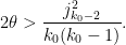
Using the known asymptotic

for  and large (see e.g. Abramowitz and Stegun), this is asymptotically of the form

or

thus giving a relationship of the form that is superior to the previous relationship .
A similar argument can be given for Theorem 5, using of the form above rather than a monomial  (and extended by zero to
  ). For future optimisation we consider a generalisation
 ![{MPZ[\varpi,\delta]}](https://s0.wp.com/latex.php?latex=%7BMPZ%5B%5Cvarpi%2C%5Cdelta%5D%7D&bg=ffffff&fg=000000&s=0&c=20201002) of in which the interval is of the form
of in which the interval is of the form  rather than , so that
  is now
  rather than
  . As before, the key point is the estimation of . The arguments leading to (22) go through for any test function , so we have to show
![\displaystyle \sum_{a_1,a_2 \in {\mathcal S}_J} \frac{k_0^{\Omega([a_1,a_2])}}{[a_1,a_2]} \int_0^\infty g^{(k_0)}(x + \frac{\log a_1}{\log R}) g^{(k_0)}(x + \frac{\log a_2}{\log R}) \frac{x^{k_0-1}}{(k_0-1)!}\ dx \leq \alpha+o(1).](https://s0.wp.com/latex.php?latex=%5Cdisplaystyle+%5Csum_%7Ba_1%2Ca_2+%5Cin+%7B%5Cmathcal+S%7D_J%7D+%5Cfrac%7Bk_0%5E%7B%5COmega%28%5Ba_1%2Ca_2%5D%29%7D%7D%7B%5Ba_1%2Ca_2%5D%7D+%5Cint_0%5E%5Cinfty+g%5E%7B%28k_0%29%7D%28x+%2B+%5Cfrac%7B%5Clog+a_1%7D%7B%5Clog+R%7D%29+g%5E%7B%28k_0%29%7D%28x+%2B+%5Cfrac%7B%5Clog+a_2%7D%7B%5Clog+R%7D%29+%5Cfrac%7Bx%5E%7Bk_0-1%7D%7D%7B%28k_0-1%29%21%7D%5C+dx+%5Cleq+%5Calpha%2Bo%281%29.+&bg=ffffff&fg=000000&s=0&c=20201002)
As has derivative equal to , this is
![\displaystyle \sum_{a_1,a_2 \in {\mathcal S}_J} \frac{k_0^{\Omega([a_1,a_2])}}{[a_1,a_2]} \int_0^{1-\frac{\log \max(a_1,a_2)}{\log R}} f'_0(x + \frac{\log a_1}{\log R}) f'_0(x + \frac{\log a_2}{\log R}) \ \ \ \ \ (30)](https://s0.wp.com/latex.php?latex=%5Cdisplaystyle+%5Csum_%7Ba_1%2Ca_2+%5Cin+%7B%5Cmathcal+S%7D_J%7D+%5Cfrac%7Bk_0%5E%7B%5COmega%28%5Ba_1%2Ca_2%5D%29%7D%7D%7B%5Ba_1%2Ca_2%5D%7D+%5Cint_0%5E%7B1-%5Cfrac%7B%5Clog+%5Cmax%28a_1%2Ca_2%29%7D%7B%5Clog+R%7D%7D+f%27_0%28x+%2B+%5Cfrac%7B%5Clog+a_1%7D%7B%5Clog+R%7D%29+f%27_0%28x+%2B+%5Cfrac%7B%5Clog+a_2%7D%7B%5Clog+R%7D%29+%5C+%5C+%5C+%5C+%5C+%2830%29&bg=ffffff&fg=000000&s=0&c=20201002)
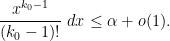
We need some sign information on  :
:
Lemma 15 On , is positive, is negative and  is positive.
Proof: From (28) we have

From construction we already know that is positive on . The above equation then shows that is negative at  , and that cannot have any local minimum in , so is negative throughout. To obtain the final claim
  we use an argument provided by Gergely Harcos in the comments: from the recursive relations for Bessel functions we can check that is a positive multiple of
  , and the claim then follows from the interlacing properties of the zeroes of Bessel functions.
Write 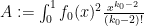 , so is positive and by Theorem 14 we have

If  , then as is negative and increasing we have

for  , and thus by change of variable
for , and thus

for all  . Similarly

for all  . By Cauchy-Schwarz we can thus bound the integral in (30) by
and so (30) reduces to
![\displaystyle \frac{j_{k_0-2}^2}{4(k_0-1)} A \sum_{a_1,a_2 \in {\mathcal S}_J} \frac{k_0^{\Omega([a_1,a_2])}}{[a_1,a_2]} (1-\frac{\log a_1}{\log R})_+^{k_0/2} (1-\frac{\log a_2}{\log R})_+^{k_0/2} \leq \alpha + o(1).](https://s0.wp.com/latex.php?latex=%5Cdisplaystyle+%5Cfrac%7Bj_%7Bk_0-2%7D%5E2%7D%7B4%28k_0-1%29%7D+A+%5Csum_%7Ba_1%2Ca_2+%5Cin+%7B%5Cmathcal+S%7D_J%7D+%5Cfrac%7Bk_0%5E%7B%5COmega%28%5Ba_1%2Ca_2%5D%29%7D%7D%7B%5Ba_1%2Ca_2%5D%7D+%281-%5Cfrac%7B%5Clog+a_1%7D%7B%5Clog+R%7D%29_%2B%5E%7Bk_0%2F2%7D+%281-%5Cfrac%7B%5Clog+a_2%7D%7B%5Clog+R%7D%29_%2B%5E%7Bk_0%2F2%7D+%5Cleq+%5Calpha+%2B+o%281%29.&bg=ffffff&fg=000000&s=0&c=20201002)
Repeating the arguments of the previous section, we can reduce this to
and by further continuing the arguments of the previous section we end up being able to take
where
Also, the previous arguments allow us to take

The key inequality (11) now becomes
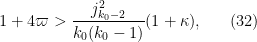
thus implies whenever (32) is obeyed with the value (31) of .

such that
.
is a function of
going to infinity with the property that
as
for all sufficiently large

144 comments
Comments feed for this article
12 September, 2013 at 4:21 pm
Gergely Harcos
In the second display below (12), should be
  .
.
[Corrected, thanks – T.]
4 October, 2013 at 11:40 am
Stijn Hanson
My apologies for all the help I’m requiring but a lot of these proof techniques are new to me in style. I’m looking at your proof of the overspill principle (Lemma 7). In the part you create your
  function to be some specific function tending to infinity with x. Thus, given any
  , the function
  will surpass it at some point. Thus:
where . Upon letting x tend to infinity
  tends to infinity and we can let m tend to infinity and we have
  and this seems clear to me.
 is a function tending to infinity with x. Then, for all natural numbers m there is some real
  such that
  . If we define
  then, surely, we must have
  whenever
  and
and 
The issue for me is the ‘sufficiently slowly’ part of the statement. Suppose that
The one thing this argument avoids is your condition of but I didn’t understand where that came from in the first place.
I’m sure I’ve missed something obvious (as I have before) but I can’t see it.
P.S. there is a slight typo in the proof in that it says “veifies” instead of “verifies”
4 October, 2013 at 12:14 pm
Terence Tao
One cannot conclude for
for  unless one already knows that
  (note that
  is not fixed, whereas (i) is only available for fixed w); this is why one needs
  to grow more slowly than
  .
.
Incidentally, in the polymath8 writeup (see https://www.dropbox.com/s/16bei7l944twojr/newgap.pdf ) the overspill principle is no longer needed, because it turns out one can take rather than have
  be a sufficiently slowly growing function of x.
4 October, 2013 at 12:43 pm
Stijn Hanson
I assumed it had something to do with that w restriction but I don’t see where comes from. The way I understand it we’re setting
  and then
  is some real number such that the
  term dips below
  whenever
  but, obviously, I must be missing something.
19 November, 2013 at 10:50 pm
Polymath8b: Bounded intervals with many primes, after Maynard | What's new
[…] this claim was already essentially established back in this Polymath8a post (or see Proposition 4.1 and Lemma 4.7 of the Polymath8a paper for essentially these bounds). In […]
31 July, 2014 at 8:33 am
Together and Alone, Closing the Prime Gap | For a better Vietnam
[…] work. At the time, though, this advance was one of the most fruitful ones. When the team filled in this piece of the puzzle on June 5, the bound on prime gaps dropped from about 4.6 million to […]
16 May, 2015 at 12:13 am
wanglaoxinr
for Cramér Conjecture ,change Pn to x, will that hold?
Pn means n th prime, Pn<Pn+1<=x, Max(Pn+1-Pn) means the maximum gap between two neighboring primes in (0,x], when x tending to infinity, Max(Pn+1-Pn)/(lnx)^2 tending to 1.
17 June, 2015 at 7:49 am
The prime tuples conjecture, sieve theory, and the work of Goldston-Pintz-Yildirim, Motohashi-Pintz, and Zhang | fragments
[…] for instance, if Conjecture 2 holds, then the number of twin primes less than should equal , where is the twin prime […]
29 October, 2015 at 8:06 pm
Alexey
I have a question about an upper bound of conjecture 2 (about k-tuple of primes). Where can I find a proof of this upper bound? How C_{k_0} depends from k_0?
Thank you
30 October, 2015 at 7:32 am
Terence Tao
This can be found for instance in the texts of Montgomery-Vaughan or Iwaniec-Kowalski, or any book on sieve theory (e.g. Friedlander-Iwaniec). I also have it as an application of the Selberg sieve in Exercise 34 of these notes.
5 April, 2016 at 9:38 pm
Where has the Time Gone? | Sublime Illusions
[…] Tao explains concepts wonderfully, especially if you want a summary of a long and intricate paper (like the explanation of Zhang Yitang’s work on the Twin Prime Conjecture and related backgroun…). Beware, not for the faint of […]
19 July, 2016 at 5:24 pm
John
Why is obvious that the Hardy-Littlewood infinite product does not converge to 0?
19 July, 2016 at 7:33 pm
John
Oh I guess it’s a simple consequence of the Prime Number Theorem and the discrete integration by part, i.e., let![f(p) = log[(1 - k/p) / (1 - 1/p)^k]](https://s0.wp.com/latex.php?latex=f%28p%29+%3D+log%5B%281+-+k%2Fp%29+%2F+%281+-+1%2Fp%29%5Ek%5D&bg=ffffff&fg=545454&s=0&c=20201002) , then one gets that the log of the HL-constant is equal to
, then one gets that the log of the HL-constant is equal to  . The latter is finite since
  is bounded above and below eventually by $0.2 n / \log n$ and $5 n / \log n$.