Kevin Ford, Ben Green, Sergei Konyagin, and myself have just posted to the arXiv our preprint “Large gaps between consecutive prime numbers“. This paper concerns the “opposite” problem to that considered by the recently concluded Polymath8 project, which was concerned with very small values of the prime gap  . Here, we wish to consider the largest prime gap
  that one can find in the interval
 ![{[X] = \{1,\dots,X\}}](https://s0.wp.com/latex.php?latex=%7B%5BX%5D+%3D+%5C%7B1%2C%5Cdots%2CX%5C%7D%7D&bg=ffffff&fg=000000&s=0&c=20201002) as
as  goes to infinity.
Finding lower bounds on  is more or less equivalent to locating long strings of consecutive composite numbers that are not too large compared to the length of the string. A classic (and quite well known) construction here starts with the observation that for any natural number
  , the consecutive numbers
  are all composite, because each
  ,
,  is divisible by some prime
  , while being strictly larger than that prime
  . From this and Stirling’s formula, it is not difficult to obtain the bound
A more efficient bound comes from the prime number theorem: there are only  primes up to , so just from the pigeonhole principle one can locate a string of consecutive composite numbers up to of length at least
  , thus
where we use  or
or  as shorthand for
  or
or  .
.
What about upper bounds? The Cramér random model predicts that the primes up to are distributed like a random subset  of density
  . Using this model, Cramér arrived at the conjecture

In fact, if one makes the extremely optimistic assumption that the random model perfectly describes the behaviour of the primes, one would arrive at the even more precise prediction
However, it is no longer widely believed that this optimistic version of the conjecture is true, due to some additional irregularities in the primes coming from the basic fact that large primes cannot be divisible by very small primes. Using the Maier matrix method to capture some of this irregularity, Granville was led to the conjecture that
(note that  is slightly larger than
  ). For comparison, the known upper bounds on are quite weak; unconditionally one has
  by the work of Baker, Harman, and Pintz, and even on the Riemann hypothesis one only gets down to
  , as shown by Cramér (a slight improvement is also possible if one additionally assumes the pair correlation conjecture; see this article of Heath-Brown and the references therein).
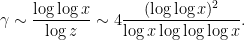
This conjecture remains out of reach of current methods. In 1931, Westzynthius managed to improve the bound (2) slightly to
which Erdös in 1935 improved to

and Rankin in 1938 improved slightly further to
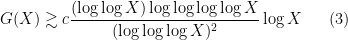
with  . Remarkably, this rather strange bound then proved extremely difficult to advance further on; until recently, the only improvements were to the constant
  , which was raised to
  in 1963 by Schönhage, to
  in 1963 by Rankin, to
  by Maier and Pomerance, and finally to
  in 1997 by Pintz.
Erdös listed the problem of making arbitrarily large one of his favourite open problems, even offering (“somewhat rashly”, in his words) a cash prize for the solution. Our main result answers this question in the affirmative:
Theorem 1 The bound (3) holds for arbitrarily large  .
.
In principle, we thus have a bound of the form

for some  that grows to infinity. Unfortunately, due to various sources of ineffectivity in our methods, we cannot provide any explicit rate of growth on at all.
We decided to announce this result the old-fashioned way, as part of a research lecture; more precisely, Ben Green announced the result in his ICM lecture this Tuesday. (The ICM staff have very efficiently put up video of his talks (and most of the other plenary and prize talks) online; Ben’s talk is here, with the announcement beginning at about 0:48. Note a slight typo in his slides, in that the exponent of  in the denominator is
  instead of
  .) Ben’s lecture slides may be found here.
By coincidence, an independent proof of this theorem has also been obtained very recently by James Maynard.
I discuss our proof method below the fold.
— 1. Sketch of proof —
Our method is a modification of Rankin’s method, combined with some work of myself and Ben Green (and of Tamar Ziegler) on counting various linear patterns in the primes. To explain this, let us first go back to Rankin’s argument, presented in a fashion that allows for comparison with our own methods. Let’s first go back to the easy bound (1) that came from using the consecutive string  of composite numbers. This bound was inferior to the prime number theorem bound (2), however this can be easily remedied by replacing
  with the somewhat smaller primorial
  , defined as the product of the primes up to and including . It is still easy to see that
  are all composite, with each
  divisible by some prime while being larger than that prime. On the other hand, the prime number theorem tells us that
  . From this, one can recover an alternate proof of (2) (perhaps not so surprising, since the prime number theorem is a key ingredient in both proofs).
This gives hope that further modification of this construction can be used to go beyond (2). If one looks carefully at the above proof, we see that the key fact used here is that the discrete interval of integers  is completely sieved out by the residue classes
  for primes , in the sense that each element in this interval is contained in at least one of these residue classes. More generally (and shifting the interval by for a more convenient normalisation), suppose we can find an interval
 ![{[y] := \{ n \in {\bf N}: n \leq y \}}](https://s0.wp.com/latex.php?latex=%7B%5By%5D+%3A%3D+%5C%7B+n+%5Cin+%7B%5Cbf+N%7D%3A+n+%5Cleq+y+%5C%7D%7D&bg=ffffff&fg=000000&s=0&c=20201002) which is completely sieved out by one residue class
which is completely sieved out by one residue class  for each
  , for some
  and
and  . Then the string of consecutive numbers
  will be composite, whenever
  is an integer larger than or equal to with
  for each prime , since each of the
  will be divisible by some prime while being larger than that prime. From the Chinese remainder theorem, one can find such an that is of size at most
  . From this and the prime number theorem, one can obtain lower bounds on if one can get lower bounds on in terms of . In particular, if for any large one can completely sieve out
 ![{[y]}](https://s0.wp.com/latex.php?latex=%7B%5By%5D%7D&bg=ffffff&fg=000000&s=0&c=20201002) with a residue class for each , and
with a residue class for each , and

then one can establish the bound (3). (The largest one can take for a given is known as the Jacobsthal function of the primorial  .) So the task is basically to find a smarter set of congruence classes than just the zero congruence classes that can sieve out a larger interval than . (Unfortunately, this approach by itself is unlikely to reach the Cramér conjecture; it was shown by Iwaniec using the large sieve that is necessarily of size
  (which somewhat coincidentally matches the Cramér bound), but Maier and Pomerance conjecture that in fact one must have
  , which would mean that the limit of this method would be to establish a bound of the form
  .)
.)
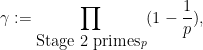
So, how can one do better than just using the “Eratosthenes” sieve ? We will divide the sieving into different stages, depending on the size of . It turns out that a reasonably optimal division of primes up to will be into the following four classes:
- Stage 1 primes: primes that are either tiny (less than
 ) or medium size (between
  and
and  ), where is a parameter to be chosen later.
- Stage 2 primes: primes that are small (between and ).
- Stage 3 primes: Primes that are very large (between
 and ).
- Stage 4 primes: Primes that are fairly large (between and ).
We will take an interval , where is given by (4), and sieve out first by Stage 1 primes, then Stage 2 primes, then Stage 3 primes, then Stage 4 primes, until none of the elements of are left.
Let’s first discuss the final sieving step, which is rather trivial. Suppose that our sieving by the first three sieving stages is so efficient that the number of surviving elements of is less than or equal to the number of Stage 4 primes (by the prime number theorem, this will for instance be the case for sufficiently large if there are fewer than  survivors). Then one can finish off the remaining survivors simply by using each of the Stage 4 primes to remove one of the surviving integers in by an appropriate choice of residue class . So we can recast our problem as an approximate sieving problem rather than a perfect sieving problem; we now only need to eliminate most of the elements of rather than all of them, at the cost of only using primes from the Stages 1-3, rather than 1-4. Note though that for given by (4), the Stage 1-3 sieving has to be reasonably efficient, in that the proportion of survivors cannot be too much larger than
  (ignoring factors of
  etc.).
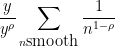
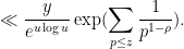
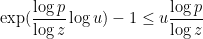
Next, we discuss the Stage 1 sieving process. Here, we will simply copy the classic construction and use the Eratosthenes sieve for these primes. The elements of that survive this process are those elements that are not divisible by any Stage 1 primes, that is to say they are only divisible by small (Stage 2) primes, or else contain at least one prime factor larger than , and no prime factors less than . In the latter case, the survivor has no choice but to be a prime in ![{(x/4,y]}](https://s0.wp.com/latex.php?latex=%7B%28x%2F4%2Cy%5D%7D&bg=ffffff&fg=000000&s=0&c=20201002) (since from (4) we have
(since from (4) we have  for large enough). In the former case, the survivor is a -smooth number – a number with no prime factors greater than . How many such survivors are there? Here we can use a somewhat crude upper bound of Rankin:
Lemma 2 Let  be large quantities, and write
  . Suppose that
Then the number of -smooth numbers in is at most  .
.
Proof: We use a Dirichlet series method commonly known as “Rankin’s trick”. Let  be a quantity to be optimised in later, and abbreviate “-smooth” as “smooth”. Observe that if is a smooth number less than , then

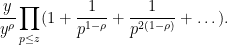
Thus, the number of smooth numbers in is at most
where we have simply discarded the constraint  . The point of doing this is that the above expression factors into a tractable Euler product
We will choose
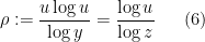
so that  and
and  . Then the above expression simplifies to
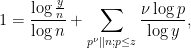
To compute the sum here, we first observe from Mertens’ theorem (discussed in this previous blog post) that
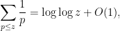
so we may bound the previous expression by
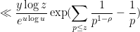
which we rewrite using (6) as
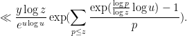
Next, we use the convexity inequality

for  and
and  , applied with
  and
and  , to conclude that
Finally, from the prime number theorem we have 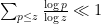 . The bound follows.
Remark 1 One can basically eliminate the  factor here (at the cost of worsening the
  error slightly to
  ) by a more refined version of the Rankin trick, based on replacing the crude bound (5) by the more sophisticated inequality

where  denotes the assertion that divides exactly
  times. (Thanks to Kevin Ford for pointing out this observation to me.) In fact, the number of -smooth numbers in is known to be asymptotically
  in the range
  , a result of de Bruijn.
In view of the error term permitted by the Stage 4 process, we would like to take as large as possible while still leaving only  smooth numbers in . A somewhat efficient choice of here is
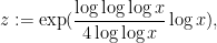
so that  and
and  , and then one can check that the above lemma does indeed show that there are smooth numbers in . (If we use the sharper bound in the remark, we can reduce the
  here to a , although this makes little difference to the final bound.) If we let
  denote all the primes in , the remaining task is then to sieve out all but of the primes in by using one congruence class from each of the Stage 2 and Stage 3 primes.
Note that is still quite large compared to the error that the Stage 4 primes can handle – it is of size about  , whereas we need to get down to a bit less than
  . Still, this is some progress (the remaining sparsification needed is of the order of
  rather than
  ).
).
For the Stage 2 sieve, we will just use a random construction, choosing uniformly at random for each Stage 2 prime. This sieve is expected to sparsify the set of survivors by a factor
which by Mertens’ theorem is of size
In particular, if is given by (4), then all the strange logarithmic factors cancel out and

In particular, we expect to be cut down to a random set (which we have called  in our paper) of size about
  . This would already finish the job for very small (e.g.
  ), and indeed Rankin’s original argument proceeds more or less along these lines. But now we want to take to be large.
Fortunately, we still have the Stage 3 primes to play with. But the number of Stage 3 primes is about  , which is a bit smaller than the number of surviving primes , which is about . So to make this work, most of the Stage 3 congruence classes need to sieve out many primes from , rather than just one or two. (Rankin’s original argument is based on sieving out one prime per congruence class; the subsequent work of Maier-Pomerance and Pintz is basically based on sieving out two primes per congruence class.)
Here, one has to take some care because the set is already quite sparse inside (its density is about ). So a randomly chosen would in fact most likely catch none of the primes in at all. So we need to restrict attention to congruence classes which already catch a large number of primes in , so that even after the Stage 2 sieving one can hope to be left with many congruence classes that also catch a large number of primes in .
Here’s where my work with Ben came in. Suppose one has an arithmetic progression  of length
  consisting entirely of primes in , and with
  a multiple of , then the congruence class
  is guaranteed to pick up at least
  primes in . My first theorem with Ben shows that no matter how large is, the set does indeed contain some arithmetic progressions
  of length . This result is not quite suitable for our applications here, because (a) we need the spacing to also be divisible by a Stage 3 prime (in our paper, we take
  for concreteness, although other choices are certainly possible), and (b) for technical reasons, it is insufficient to simply have a large number of arithmetic progressions of primes strewn around ; they have to be “evenly distributed” in some sense in order to be able to still cover most of after throwing out any progression that is partly or completely sieved out by the Stage 2 primes. Fortunately, though, these distributional results for linear equations in primes were established by a subsequent paper of Ben and myself, contingent on two conjectures (the Mobius-Nilsequences conjecture and the inverse conjecture for the Gowers norms) which we also proved (the latter with Tamar Ziegler) in some further papers. (Actually, strictly speaking our work does not quite cover the case needed here, because the progressions are a little “narrow”; we need progressions of primes in whose spacing is comparable to instead of , whereas our paper only considered the situation in which the spacing was comparable to the elements of the progression. It turns out though that the arguments can be modified (somewhat tediously) to extend to this case though.)


44 comments
Comments feed for this article
21 August, 2014 at 11:49 am
Anonymous
Is there a way to get the pdf files of ICM proceedings of this year online?
Thanks
21 August, 2014 at 7:22 pm
Terence Tao
I would imagine that they will eventually be available at http://www.mathunion.org/ICM/ . But one may have to wait some weeks or perhaps months before they are all done with the typesetting etc..
21 August, 2014 at 10:47 pm
Gil Kalai
For ICM2010 it took about two years for the proceedings to become freely available in the above site. Meanwhile about 50 of the ICM 2014 proceedings’ contributions are already available on arXiv, via this search.http://arxiv.org/find/all/1/co:+icm/0/1/0/all/0/1 (I got it from Peter Woit’s blog.) Videos of lectures can already be found here. http://www.icm2014.org/en/vod/vod
22 August, 2014 at 5:58 am
Hyun Woo Kwon
I’m a technical Editor on this year ICM Proceedings. Actually, they are already given in USB except for plenary lectures. “USB” is given to participants. I’m not sure when it will be uploaded in IMU websites.
21 August, 2014 at 12:02 pm
Ben Green
I understand James Maynard’s preprint will be appearing later today. There is a sense in which he uses progress on small prime gaps to say something about large prime gaps! The method is quite different to ours, so it is remarkable that these papers should appear within a day of one another after a 75-year wait.
21 August, 2014 at 6:05 pm
Gergely Harcos
Maynard’s preprint is up (http://arxiv.org/abs/1408.5110). Congratulations to all of you!
21 August, 2014 at 7:16 pm
Pace Nielsen
Ben Green’s announcement talk at the ICM was very interesting. One of the things that stuck out to me most was his statement about double ineffectivity [I think this was in answer to a question after the talk(?)], so I was looking to see if James could get around that. It looks like he has!
21 August, 2014 at 10:02 pm
Gil Kalai
Congratulations!
22 August, 2014 at 2:38 am
BQ
Yes, I think more people should announce their results in this old-fashioned way — by giving a plenary lecture at ICM.
22 August, 2014 at 6:16 am
interested non-expert
Congratulations to all authors! As Ben Green pointed out, it is a strange coincidence that your team and James Maynard found a proof at the same time (after 75years). Some questions:
1) Has there been a major breakthrough recently, which both of you have used? What are other explanations?
2) What are the major differences between your proofs and conclusions? Are the involved/developed methods of the similar powerful?
3) As in the case for small gaps, which is a special case of a weaker variant of a great unknown conjecture (twin-prime conjecture), is there an analog for large primes?
Thanks!!
22 August, 2014 at 6:37 am
Terence Tao
Both of our papers need some recent results on how to catch primes inside arithmetic progressions, but we use different results. The paper of Kevin, Ben, Sergei and myself use the results of Ben and myself (and of Tamar Ziegler) on linear equations in primes to locate arithmetic progressions that consist solely of primes. James’ argument instead uses a variant of his result on admissible prime tuples that can catch many primes but are also allowed to catch composites (in particular, he uses the same engine to establish both small gaps between primes and large gaps between primes, which is a pleasing symmetry). The latter has the advantage of coming with explicit bounds (the Siegel zero ineffectivity issue is still present, due to the reliance on the Bombieri-Vinogradov theorem, but there are ways to deal with the exceptional zero, e.g. via effective variants of Bombieri-Vinogradov). On the other hand, the sieving process in our paper is a bit simpler to analyse than the one in James’ paper, although they are broadly both of Erdos-Rankin type. There is a good chance that one can combine the most efficient parts of both papers to obtain a cleaner proof of the result that also provides a better bound; we’re looking into that right now.
The analogue of the twin prime conjecture here is probably the Cramer conjecture (although the obstruction to solving the latter is different, it is the sheer difficulty of locating very rare events, rather than the parity problem). This conjecture is well out of reach of any of the Erdos-Rankin-based methods (which have a natural limit at , stopping well short of the Cramer prediction
  ).
).
23 August, 2014 at 1:26 pm
Polymath 8 – a Success! | Combinatorics and more
[…] Update (August 23): Before moving to small gaps, Sound’s 2007 survey briefly describes the situation for large gaps. The Cramer probabilistic heuristic suggests that there are consecutive primes in [1,n] which are apart, but not apart where c and C are some small and large positive constants. It follows from the prime number theorem that there is a gap of at least . And there were a few improvements in the 30s ending with a remarkable result by Rankin who showed that there is a gap as large as times . Last week Kevin Ford, Ben Green, Sergei Konyagin, and Terry Tao and independently James Maynard were able to improve Rankin’s estimate by a function that goes to infinity with n. See this post on “What’s new.” […]
24 August, 2014 at 7:05 am
jozsef
I was wondering if there is a two-sided variant of the result; if there are primes so that the nearest prime, above or below, is far.
24 August, 2014 at 7:47 am
Terence Tao
This looks likely; a result of this form (with a weaker gap bound) was established by Erdos back in 1949, and in 1981 Maier (using his famous matrix method) established this result with a Rankin-type gap bound (in fact he could get k consecutive large prime gaps for any fixed k). It looks likely that our arguments can be combined with Maier’s, but there are some technical issues to sort out; we’re planning to look into this question soon.
24 August, 2014 at 7:59 am
math stat
Hi Professor Tao;
1. There is no Granville conjecture, which improves the Cramer conjecture, he said himself on Mathoverflow.
2. Why there is no specific bound for G(X) given? The PNT should implies that G(X) < 0 small.
3. Does the Jacothal function implies that G(X) << (log X)^2 ?
Thank you.
[Wordpress interprets any text between < and > as HTML and deletes it. Use < and > instead. -T.]
24 August, 2014 at 9:57 am
Terence Tao
1. Granville did not make a conjecture for the precise value of , but he did make the conjecture that this limsup will be at least
  (see the bottom of page 12 of his paper here).
2. (See formatting note above.)
3. I am presuming that the intended question here is whether one can use known or conjectural bounds on the Jacobsthal function to imply that . Unfortunately this does not appear to be the case. The Jacobsthal function lets one control one special type of prime gap, caused by a string of consecutive numbers that each have a quite small prime factor (of size comparable to the logarithm of the numbers in the string). However, it does not say anything much about other prime gaps, that is to say strings of composite numbers, some of which contain large prime factors instead of small ones. The Cramer model suggests that the gaps with
  will be of this latter type and will thus be out of reach of constructions based on the Jacobsthal function. (Maier and Pomerance have a probabilistic heuristic bound on the Jacobsthal function that suggests that the largest prime gap that can be created from optimisers to that function is of size at most
  , but this is not expected to be the true value of
  , merely the limit of this method.)
24 August, 2014 at 9:18 pm
Janko Bračič
Dear Professor Tao,
I have a question which is not directly related to the topic of this blog, but it is about the pairs of primes. Maybe the question is easy for an expert however I am not able to find an answer.
Question: Let be an integer. What is the best known upper bound for number of pairs
  up to
up to  , i.e.,
  , such that
  and
and  both are primes?
Thank you!
24 August, 2014 at 11:32 pm
Ben Green
I think about 4 times the expected truth of $c X/\log^2 X$ is a well-known exercise in sieve theory. The 4 has been improved to about 3.4 using much more elaborate sieve theoretic methods. Here is a free to view reference for these matters in the case $d = 2$: http://arxiv.org/pdf/1205.0774.pdf
25 August, 2014 at 1:39 am
Janko Bračič
Thank you for the answer and the link!
25 August, 2014 at 6:11 pm
dwu
Hi Professor Tao:
I had a question about the particular choice of the division of the primes into these four separate classes or stages.
It’s quite understandable from the paper and from the above proof sketch how these sets of primes are used effectively to sieve out the desired interval, but is there any easily-explainable intuition for why this particular division is more effective than other known approaches for choosing residue classes? At a superficial level, it seems rather strange that one would want to partition the primes in this way, with one of the sets even being composed of two disjoint intervals, namely the stage 1 primes for which we simply choose the zero residue class.
Is the choice of these four stages mostly just an artifact of trying to exploit the tools we have available at the moment (e.g. strong bounds on the density of smooth numbers), or is there a more fundamental reason? For example, if one could actually find the optimal or a near-optimal selection of the residue classes for this sieve, would one broadly expect it to bear any similarities to the construction here?
26 August, 2014 at 10:40 pm
Terence Tao
I would say that this is primarily an artifact of trying to optimise between the known reasonably effective sieving methods we have (random, greedy, Eratosthenes). We chose the Stage 1 (Eratosthenes sieve) primes to be disconnected because it had the convenient consequence that the sifted set was essentially the set of primes (as opposed to almost primes, which is what would have happened if we did not include the tiny primes into this stage), so we could (almost) use off-the-shelf theorems about primes. But these theorems are likely also true for almost primes, and one would probably get comparable results if the tiny primes were shifted into Stage 2 (incidentally, this is basically what Maynard does in his paper; also, his Stage 2 uses a shifted Eratosthenes sieve instead of a random sieve, and this also gives comparable results although it requires a bit more sieve theory to analyse).
There isn’t much known as to what the truly optimal sieving process is – there is no known practical algorithm for locating these things once the size of the interval gets even moderately large. Even if the exact optimisers were known numerically, they could end up being rather unedifying – the problem is so combinatorially complicated that there is no particular reason to suspect any particularly nice structure to the exact optimiser. (There might be an interestingly structured quasi-optimiser, though, even if it is technically “beaten” by some semi-random set of congruence classes that manages by pure chance to beat the structured quasi-optimiser by a little bit.)
27 August, 2014 at 2:48 pm
Billy
Dear Professor Tao
Click to access 38128.pdf
In the above link which shows a one-page paper it is stated that
“the density of Chen primes gradually thins” . Is this enough to prove that there exist infinite non-Chen primes ? Or does the conclusion that there are infinite non-Chen primes come some way from the infinity of Chen primes in arithmetic progression, proved by you and B.Green?
Any proof that there is an infinite number of non-Chen primes could help me significantly proceed with an attempt of proving a conjecture that I ve been working on as an amateur for a long time.
Thank you in advance
27 August, 2014 at 3:59 pm
Terence Tao
The set of Chen primes has a significantly smaller density than the set of all primes. For instance, a minor modification of the proof of Brun’s theorem shows that the sum of reciprocals of the Chen primes is convergent, whereas the sum of the reciprocals of all the primes is divergent. More quantitatively, for large , the number of primes up to
  is approximately
  (the prime number theorem), but standard sieve theory techniques (e.g the Selberg sieve) show that the number of Chen primes up to
  is
is  , which is asymptotically smaller. (Technically, this depends on whether one permits one of the prime factors of the Chen prime to be small or not. If one allows small prime factors, the bound is actually a little bit bigger, namely
  .)
.)
28 August, 2014 at 2:24 pm
Billy
Thank you very much professor Tao.
Should I finish my attempt of proving the conjecture, to which mathematical union should I send my work to get its validity examined ?
31 August, 2014 at 12:09 am
Philip Lee
I am just a science student, and I am not very familiar with deep maths. I don’t quite see how the prime number theorem could give such a tight bound that can lead to a pigeonhole principle, just by itself. It seems clear that anomalous clusters of primes becomes well, anomalous, but we see that the PNT is an asymptotic result. Anyone care to give a short explanation, if possible? Prime numbers make very interesting work.
31 August, 2014 at 8:49 am
Terence Tao
Suppose for instance that one knows that there are at most 99 primes in the interval (this is asymptotically the type of information one gets from the prime number theorem, replacing 99 and 1000 with larger numbers). We can divide the interval
  into 100 intervals of
  of length 10. By the pigeonhole principle (applied in the opposite direction to its traditional formulation), at least one of these intervals must be completely devoid of primes, giving rise to a prime gap of size at least 11.
31 August, 2014 at 10:01 pm
Philip Lee
Thanks for the reply. I wasn’t thinking about limits as I did not see the inequality with the tilde, which has a little o(1) in it (so the inequality depends on precision, or the smallness of 1/”1000″).
31 August, 2014 at 1:52 am
Thomas Dybdahl Ahle
“where grows to infinity” – I suppose you could write that as
  then? since you already use
  for sub-constants.
31 August, 2014 at 8:57 am
Terence Tao
Yes, although this can cause some conflict in analytic number theory because is also used to denote the number of prime divisors of
  . (Admittedly, we don’t use that notation in this particular paper, but it shows up often enough in other analytic number theory papers that it can lead to confusion if we use it here. Given that it is only needed once in our paper, we felt that it was not worth introducing a notation for it, even if it is standard in some fields of mathematics.)
1 September, 2014 at 6:53 am
interested non-expert
This week, an article dealing with prime/natural number networks has been published in a serious physics journal: http://journals.aps.org/pre/abstract/10.1103/PhysRevE.90.022806 It also deals with the Cramer-conjecture on large gaps between primes. As it seem to be partially connected with the statistical analysis in this blog-article, I wonder what are the connections and whether it presents new insights? Thanks alot!
4 September, 2014 at 6:53 pm
curious non-expert
Does this relate to Perron Frobenius properties of stochastic matrices? I am at a level of non-expertise that it seems incredible that a theorem like PF could be proved. The up-shot, as I see it, is that for mixing to occur in a network and reach a static steady state, all cycles in the network should have lengths which have their gcd = 1. This is kind of like factoring. What about random stochastic matrices? What about a steady state for the grown network with a ‘prime’ law distribution for the links. It would seem that half the numbers have a prime factor of two, some other fraction with a factor of 3, and so on. Is there an efficient method to label the nodes in the network? It turns out the combinatorix and discrete structures, and complex and asymptotic analysis have a deep connection (I guess the series representation (harmonics), and generating functions are quite natural for those fields). As with all curious people, I have my own other ideas on the representation of primes and the entropy for the set of primes.
Knowing so little, and might being so wrong, it can look like that I am a very strange troll from the internet.
5 September, 2014 at 3:44 pm
Anonymous
Terry, where is your paper submitted to?
16 December, 2014 at 8:29 pm
Long gaps between primes | What's new
[…] gaps between primes“. This is a followup work to our two previous papers (discussed in this previous post), in which we had simultaneously shown that the maximal […]
27 December, 2014 at 2:45 pm
billy
Dear professor Tao
If one divides the set of natural numbers into smaller sets based on their divisibility with a random prime number p , what he gets are p sequences of natural numbers of which only p-1 can contain prime numbers.For example, dividing all natural numbers with 5, will produce 5 sequences,
containing numbers of the form 5k+1 or 5k+2 or 5k+3 or 5k+4 or 5k.
Of course, a prime can only belong in one of the first four mentioned sequences.
So, my question is:
Are prime numbers equally distributed in those 4 sequences ?
For instance is 1 prime per 4 of the form 5k+1?
Or is 1 prime per 12 of the form 13k+7?
In general is there any proof that 1 prime per p-1 is of the form pk+b
where p is a prime
k is a natural number and
b is a natural number smaller than p ?
[Yes, this is the prime number theorem in arithmetic progressions, discussed for instance in the recent post https://terrytao.wordpress.com/2014/12/09/254a-notes-2-complex-analytic-multiplicative-number-theory/ . See also Dirichlet’s theorem, http://en.wikipedia.org/wiki/Dirichlet%27s_theorem_on_arithmetic_progressions -T.]
28 December, 2014 at 6:25 am
Carl L. Lambert
See #PrimeNumberGuy tweets on Twitter for a simple view of consecutive composite numbers, including groups of trillions of such consecutive composites in the mega number ranges.
22 February, 2015 at 3:16 pm
Fan
Prof. Tao
I’m confused about your definition of z-smooth numbers. For one, it is quite opposite what the wiki page you linked to says. For the other, after stage 1 of the sieve what is left should be smooth numbers as defined by Wikipedia rather than your definition.
[A typo, now corrected – T.]
22 February, 2015 at 3:22 pm
Fan
What is the x in Lemma 2? Is it the same as before or a typo?
[A typo, now corrected – T.]
22 February, 2015 at 8:14 pm
Fan
Nice article. Only kind of lost on the last paragraph.
10 October, 2015 at 7:30 pm
Abhishek
I would like to understand the choice of \rho . In particular, is there any reason to set \rho = log(u)/log(z) in the Proof of the Rankin Trick.
10 October, 2015 at 9:28 pm
Terence Tao
One can try other choices of , but they lead to poorer bounds; the choice given is the one which optimises the bound for the given method.
28 February, 2016 at 9:20 pm
Are there arbitrarily large gaps between consecutive primes? – math.stackexchange.com #JHedzWorlD | JHedzWorlD
[…] $g$, then you should look at integers $leq e^sqrtg$ (which, for $g = 10000$ is pretty large). See this post of Terence Tao for […]
18 May, 2017 at 12:00 pm
Gaps between prime-like sets | google-site-verification: google1edf67008356a9e1.html
[…] This post was inspired by a question of Trevor Wooley after a talk of James Maynard at MSRI. He asked what was known for lower bounds of large gaps between integers that have a representation as the sum of two squares. This posts assume some familiarity with the large gaps between primes problem. […]
13 September, 2017 at 2:48 pm
M.F.
I find it strange, ambiguous, and confusing to write “log A(log B) “. If you mean “(log A) log B” the (..) should be around the first factor. If you don’t mean this, then you must mean ” log (A log B) “, so why don’t you choose this unambiguous way of writing it? The chosen variant “log A(log B)” is no better than ” log A log B” without parentheses (and actually the latter is more likely understood (correctly?) as (log A) log B than the former). Just wondering — with all due respect!
[Typo corrected, thanks – T.]
19 August, 2020 at 4:20 am
Carl L. Lambert
To: Terrence Tao, August 19, 2020
The Lambert Prime Number Formula not only produces all the prime numbers and eliminates all the composite numbers, but it also can produce all the consecutive composite number clusters. Try this:
n * p# + v or n * p# – v
… where n is any integer between 0 and infinity, the * is the multiplication
symbol, and # indicates the primorial function, and p is any prime number.
Now then, simply assign any value to v between 2 and p+1, inclusive, and a composite number will be produced, which means that, for any value of n and any particular value of p, all those values for v constitute a contiguous composite number cluster consisting of p number of composite numbers (plus more when smaller clusters are enveloped by larger clusters in the larger number ranges). This is well covered in my Treatise #9, “The Mirror Images of Contiguous Composite Number Clusters”, 2015. It is not necessary to play with factorials here because all the prime numbers used in a primorial provide all the necessary divisors to be used either side of the plus (or minus) sign to prove a result of the expression to be composite.
Example:
n * 223092827# + v
produces an infinite number of contiguous composite number clusters, each consisting of 223092827 consecutive composite numbers and
n * 223092827# – v
produces a different but also infinite number of contiguous composite number clusters, each consisting of 223092827 consecutive composite numbers.
Carl L. Lambert
#PrimeNumberGuy