
You are currently browsing the tag archive for the ‘algebraic varieties’ tag.
Louis Esser, Burt Totaro, Chengxi Wang, and myself have just uploaded to the arXiv our preprint “Varieties of general type with many vanishing plurigenera, and optimal sine and sawtooth inequalities“. This is an interdisciplinary paper that arose because in order to optimize a certain algebraic geometry construction it became necessary to solve a purely analytic question which, while simple, did not seem to have been previously studied in the literature. We were able to solve the analytic question exactly and thus fully optimize the algebraic geometry construction, though the analytic question may have some independent interest.
Let us first discuss the algebraic geometry application. Given a smooth complex 


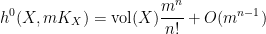
 for some non-negative number
  , which is called the volume of the variety , which is an invariant that reveals some information about the birational geometry of . For instance, if the canonical line bundle is ample (or more generally, nef), this volume is equal to the intersection number
  (roughly speaking, the number of common zeroes of generic sections of the canonical line bundle); this is a special case of the asymptotic Riemann-Roch theorem. In particular, the volume is a natural number in this case. However, it is possible for the volume to also be fractional in nature. One can then ask: how small can the volume get without vanishing entirely? (By definition, varieties with non-vanishing volume are known as varieties of general type.)
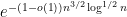
It follows from a deep result obtained independently by Hacon–McKernan, Takayama and Tsuji that there is a uniform lower bound for the volume 


The space 


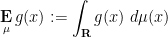
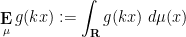
Now it is time to turn to the analytic side of the paper by describing the optimization problem that we solve. We consider the sawtooth function ![{g: {\bf R} \rightarrow (-1/2,1/2]}](https://s0.wp.com/latex.php?latex=%7Bg%3A+%7B%5Cbf+R%7D+%5Crightarrow+%28-1%2F2%2C1%2F2%5D%7D&bg=ffffff&fg=000000&s=0&c=20201002)

![{(-1/2,1/2]}](https://s0.wp.com/latex.php?latex=%7B%28-1%2F2%2C1%2F2%5D%7D&bg=ffffff&fg=000000&s=0&c=20201002)


 is bounded above by
  , we certainly have the trivial bound
 could attain the value of is if the probability measure was supported on half-integers, but in that case
  would vanish. For the algebraic geometry application discussed above one is then led to the following question: for a given choice of , what is the best upper bound
  on the quantity
 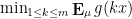 that holds for all probability measures ?
If one considers the deterministic case in which 


 . Thus we have
  is comparable to
  . In fact we were able to compute this quantity precisely:
Theorem 1 (Optimal bound for sawtooth inequality) Let.
In particular, we have
- (i) If
for some natural number
, then
.
- (ii) If
for some natural number
.
as
We establish this bound through duality. Indeed, suppose we could find non-negative coefficients 
 . Integrating this against an arbitrary probability measure , we would conclude
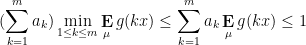
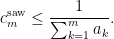 by selecting suitable candidate measures and computing the means
  . The theory of linear programming duality tells us that this method must give us the optimal bound, but one has to locate the optimal measure and optimal weights . This we were able to do by first doing some extensive numerics to discover these weights and measures for small values of , and then doing some educated guesswork to extrapolate these examples to the general case, and then to verify the required inequalities. In case (i) the situation is particularly simple, as one can take to be the discrete measure that assigns a probability
  to the numbers
  and the remaining probability of
  to
to  , while the optimal weighted inequality (1) turns out to be
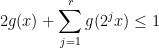
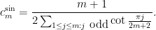
After solving the sawtooth problem, we became interested in the analogous question for the sine function, that is to say what is the best bound 
 Fourier coefficients of . To our knowledge this quantity has not previously been studied in the Fourier analysis literature. By adopting a similar approach as for the sawtooth problem, we were able to compute this quantity exactly also:
Theorem 2 For anyIn particular,
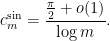
Interestingly, a closely related cotangent sum recently appeared in this MathOverflow post. Verifying the lower bound on 


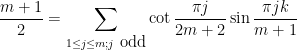 , first posed by Eisenstein in 1844 and proved by Stern in 1861. The upper bound arises from establishing the trigonometric inequality
 , which to our knowledge is new; the left-hand side has a Fourier-analytic intepretation as convolving the Fejér kernel with a certain discretized square wave function, and this interpretation is used heavily in our proof of the inequality.
In 1946, Ulam, in response to a theorem of Anning and Erdös, posed the following problem:
Problem 1 (Erdös-Ulam problem) Let
be a set such that the distance between any two points in
is rational. Is it true that
?
The paper of Anning and Erdös addressed the case that all the distances between two points in
The Erdös-Ulam problem remains open; it was discussed recently over at Gödel’s lost letter. It is in fact likely (as we shall see below) that the set
The main tool of the Solymosi-de Zeeuw analysis was Faltings’ celebrated theorem that every algebraic curve of genus at least two contains only finitely many rational points. The purpose of this post is to observe that an affirmative answer to the full Erdös-Ulam problem similarly follows from the conjectured analogue of Falting’s theorem for surfaces, namely the following conjecture of Bombieri and Lang:
Conjecture 2 (Bombieri-Lang conjecture) Let
which is of general type. Then the set
of rational points of
In fact, the Bombieri-Lang conjecture has been made for varieties of arbitrary dimension, and for more general number fields than the rationals, but the above special case of the conjecture is the only one needed for this application. We will review what “general type” means (for smooth projective complex varieties, at least) below the fold.
The Bombieri-Lang conjecture is considered to be extremely difficult, in particular being substantially harder than Faltings’ theorem, which is itself a highly non-trivial result. So this implication should not be viewed as a practical route to resolving the Erdös-Ulam problem unconditionally; rather, it is a demonstration of the power of the Bombieri-Lang conjecture. Still, it was an instructive algebraic geometry exercise for me to carry out the details of this implication, which quickly boils down to verifying that a certain quite explicit algebraic surface is of general type (Theorem 4 below). As I am not an expert in the subject, my computations here will be rather tedious and pedestrian; it is likely that they could be made much slicker by exploiting more of the machinery of modern algebraic geometry, and I would welcome any such streamlining by actual experts in this area. (For similar reasons, there may be more typos and errors than usual in this post; corrections are welcome as always.) My calculations here are based on a similar calculation of van Luijk, who used analogous arguments to show (assuming Bombieri-Lang) that the set of perfect cuboids is not Zariski-dense in its projective parameter space.
We also remark that in a recent paper of Makhul and Shaffaf, the Bombieri-Lang conjecture (or more precisely, a weaker consequence of that conjecture) was used to show that if
Let us now give the elementary reductions to the claim that a certain variety is of general type. For sake of contradiction, let 


Given any two points 


Now take four points 


for 


By inspecting the projection 


Claim 3 For any non-zero rational
in general position, the rational points of the affine surface
is not Zariski dense in
This is already very close to a claim that can be directly resolved by the Bombieri-Lang conjecture, but
![\displaystyle \overline{V} := \{ [X,Y,Z,R_1,R_2,R_3,R_4] \in {\bf CP}^6: Q(X,Y,Z,R_1,R_2,R_3,R_4) = 0 \} \ \ \ \ \ (1)](https://s0.wp.com/latex.php?latex=%5Cdisplaystyle+%5Coverline%7BV%7D+%3A%3D+%5C%7B+%5BX%2CY%2CZ%2CR_1%2CR_2%2CR_3%2CR_4%5D+%5Cin+%7B%5Cbf+CP%7D%5E6%3A+Q%28X%2CY%2CZ%2CR_1%2CR_2%2CR_3%2CR_4%29+%3D+0+%5C%7D+%5C+%5C+%5C+%5C+%5C+%281%29&bg=ffffff&fg=000000&s=0&c=20201002)
of 

with

and the projective complex space 
![{[X,Y,Z,R_1,R_2,R_3,R_4]}](https://s0.wp.com/latex.php?latex=%7B%5BX%2CY%2CZ%2CR_1%2CR_2%2CR_3%2CR_4%5D%7D&bg=ffffff&fg=000000&s=0&c=20201002)


![{\{ [X,Y,0,R_1,R_2,R_3,R_4]: X^2+bY^2=R^2; R_j = \pm R_1 \hbox{ for } j=2,3,4\}}](https://s0.wp.com/latex.php?latex=%7B%5C%7B+%5BX%2CY%2C0%2CR_1%2CR_2%2CR_3%2CR_4%5D%3A+X%5E2%2BbY%5E2%3DR%5E2%3B+R_j+%3D+%5Cpm+R_1+%5Chbox%7B+for+%7D+j%3D2%2C3%2C4%5C%7D%7D&bg=ffffff&fg=000000&s=0&c=20201002)
![{[X,Y,Z,R_1,R_2,R_3,R_4] \mapsto [X,Y,Z]}](https://s0.wp.com/latex.php?latex=%7B%5BX%2CY%2CZ%2CR_1%2CR_2%2CR_3%2CR_4%5D+%5Cmapsto+%5BX%2CY%2CZ%5D%7D&bg=ffffff&fg=000000&s=0&c=20201002)
Heuristically, the reason why we expect few rational points in 


this is a convergent sum if
The Bombieri-Lang conjecture, Conjecture 2, can be viewed as a formalisation of the above heuristics (roughly speaking, it is one of the most optimistic natural conjectures one could make that is compatible with these heuristics while also being invariant under birational equivalence).
Unfortunately,

for 


![{[X,Y,Z]}](https://s0.wp.com/latex.php?latex=%7B%5BX%2CY%2CZ%5D%7D&bg=ffffff&fg=000000&s=0&c=20201002)
![{[x_j,y_j,1]}](https://s0.wp.com/latex.php?latex=%7B%5Bx_j%2Cy_j%2C1%5D%7D&bg=ffffff&fg=000000&s=0&c=20201002)


The other way in which could occur is if a non-trivial linear combination of at least two of the gradient vectors vanishes. From (2), this can only occur if 


for two choices of sign 


![\displaystyle [X,Y,Z,R_1,R_2,R_3,R_4] = [\pm \sqrt{b} i, 1, 0, 0, 0, 0, 0]. \ \ \ \ \ (5)](https://s0.wp.com/latex.php?latex=%5Cdisplaystyle+%5BX%2CY%2CZ%2CR_1%2CR_2%2CR_3%2CR_4%5D+%3D+%5B%5Cpm+%5Csqrt%7Bb%7D+i%2C+1%2C+0%2C+0%2C+0%2C+0%2C+0%5D.+%5C+%5C+%5C+%5C+%5C+%285%29&bg=ffffff&fg=000000&s=0&c=20201002)
If the non-trivial linear combination involved three or more gradient vectors, then by the pigeonhole principle at least two of the signs involved must be equal, and so the only singular points are (5). So the only remaining possibility is when we have two gradient vectors 


We will shortly show that the 

This will be done below the fold, by the pedestrian device of explicitly constructing global differential forms on
I thank Mark Green and David Gieseker for helpful conversations (and a crash course in varieties of general type!).
Remark 5 The above argument shows in fact (assuming Bombieri-Lang) that sets
, we obtain a similar conclusion with “rational” replaced by “lying in
[Note: the idea for this post originated before the recent preprint of Mochizuki on the abc conjecture was released, and is not intended as a commentary on that work, which offers a much more non-trivial perspective on scheme theory. -T.]
In classical algebraic geometry, the central object of study is an algebraic variety 
- (Algebraic geometry) One can view a variety through the set
of points (over
- (Commutative algebra) One can view a variety through the field of rational functions
on that variety, or the subring
of polynomial functions in that field.
- (Dual algebraic geometry) One can view a variety through a collection of polynomials
that cut out that variety.
- (Dual commutative algebra) One can view a variety through the ideal
of polynomials that vanish on that variety.
For instance, the unit circle over the reals can be thought of in each of these four different ways:
- (Algebraic geometry) The set of points
.
- (Commutative algebra) The quotient
of the polynomial ring
by the ideal generated by
(or equivalently, the algebra generated by
subject to the constraint
), or the fraction field of that quotient.
- (Dual algebraic geometry) The polynomial
- (Dual commutative algebra) The ideal
generated by
The four viewpoints are almost equivalent to each other (particularly if the underlying field
Because of the connections between these viewpoints, there are extensive “dictionaries” (most notably the ideal-variety dictionary) that convert basic concepts in one of these four perspectives into any of the other three. For instance, passing from a variety to a subvariety shrinks the set of points and the function field, but enlarges the set of polynomials needed to cut out the variety, as well as the associated ideal. Taking the intersection or union of two varieties corresponds to adding or multiplying together the two ideals respectively. The dimension of an (irreducible) algebraic variety can be defined as the transcendence degree of the function field, the maximal length of chains of subvarieties, or the Krull dimension of the ring of polynomials. And so on and so forth. Thanks to these dictionaries, it is now commonplace to think of commutative algebras geometrically, or conversely to approach algebraic geometry from the perspective of abstract algebra. There are however some very well known defects to these dictionaries, at least when viewed in the classical setting of algebraic varieties. The main one is that two different ideals (or two inequivalent sets of polynomials) can cut out the same set of points, particularly if the underlying field 


![{{\bf R}[x]}](https://s0.wp.com/latex.php?latex=%7B%7B%5Cbf+R%7D%5Bx%5D%7D&bg=ffffff&fg=000000&s=0&c=20201002)


![{{\bf C}[x]}](https://s0.wp.com/latex.php?latex=%7B%7B%5Cbf+C%7D%5Bx%5D%7D&bg=ffffff&fg=000000&s=0&c=20201002)
Nowadays, the standard way to deal with these issues is to replace the notion of an algebraic variety with the more general notion of a scheme. Roughly speaking, the way schemes are defined is to focus on the commutative algebra perspective as the primary one, and to allow the base field
Thus, for instance, in scheme theory the rings ![{{\bf R}[x]/(x^2)}](https://s0.wp.com/latex.php?latex=%7B%7B%5Cbf+R%7D%5Bx%5D%2F%28x%5E2%29%7D&bg=ffffff&fg=000000&s=0&c=20201002)
![{{\bf R}[x]/(x)}](https://s0.wp.com/latex.php?latex=%7B%7B%5Cbf+R%7D%5Bx%5D%2F%28x%29%7D&bg=ffffff&fg=000000&s=0&c=20201002)


Because of this, it seems that the link between the commutative algebra perspective and the algebraic geometry perspective is still not quite perfect in scheme theory, unless one is willing to start “fattening” various varieties to correctly model multiplicity or singularity. But – and this is the trivial remark I wanted to make in this blog post – one can recover a tight connection between the two perspectives as long as one allows the freedom to arbitrarily extend the underlying base ring.
Here’s what I mean by this. Consider classical algebraic geometry over some commutative ring 
![{P_1,\ldots,P_m \in R[x_1,\ldots,x_d]}](https://s0.wp.com/latex.php?latex=%7BP_1%2C%5Cldots%2CP_m+%5Cin+R%5Bx_1%2C%5Cldots%2Cx_d%5D%7D&bg=ffffff&fg=000000&s=0&c=20201002)


![\displaystyle = \{P_1Q_1+\ldots+P_mQ_m: Q_1,\ldots,Q_m \in R[x_1,\ldots,x_d]\}](https://s0.wp.com/latex.php?latex=%5Cdisplaystyle++%3D+%5C%7BP_1Q_1%2B%5Cldots%2BP_mQ_m%3A+Q_1%2C%5Cldots%2CQ_m+%5Cin+R%5Bx_1%2C%5Cldots%2Cx_d%5D%5C%7D&bg=ffffff&fg=000000&s=0&c=20201002)
in ![{R[x_1,\ldots,x_d]}](https://s0.wp.com/latex.php?latex=%7BR%5Bx_1%2C%5Cldots%2Cx_d%5D%7D&bg=ffffff&fg=000000&s=0&c=20201002)
![\displaystyle V[R] := \{ (y_1,\ldots,y_d) \in R^d: P_1(y_1,\ldots,y_d) = \ldots = P_m(y_1,\ldots,y_d) = 0 \},](https://s0.wp.com/latex.php?latex=%5Cdisplaystyle++V%5BR%5D+%3A%3D+%5C%7B+%28y_1%2C%5Cldots%2Cy_d%29+%5Cin+R%5Ed%3A+P_1%28y_1%2C%5Cldots%2Cy_d%29+%3D+%5Cldots+%3D+P_m%28y_1%2C%5Cldots%2Cy_d%29+%3D+0+%5C%7D%2C&bg=ffffff&fg=000000&s=0&c=20201002)
since each of the polynomials 
![{V[R]}](https://s0.wp.com/latex.php?latex=%7BV%5BR%5D%7D&bg=ffffff&fg=000000&s=0&c=20201002)

![\displaystyle V[R] := \{ (y_1,\ldots,y_d) \in R^d: P(y_1,\ldots,y_d) = 0 \hbox{ for all } P \in I \}.](https://s0.wp.com/latex.php?latex=%5Cdisplaystyle++V%5BR%5D+%3A%3D+%5C%7B+%28y_1%2C%5Cldots%2Cy_d%29+%5Cin+R%5Ed%3A+P%28y_1%2C%5Cldots%2Cy_d%29+%3D+0+%5Chbox%7B+for+all+%7D+P+%5Cin+I+%5C%7D.&bg=ffffff&fg=000000&s=0&c=20201002)
Thus the ideal ![{V_I[R]}](https://s0.wp.com/latex.php?latex=%7BV_I%5BR%5D%7D&bg=ffffff&fg=000000&s=0&c=20201002)


![\displaystyle V[R'] := \{ (y_1,\ldots,y_d) \in (R')^d:](https://s0.wp.com/latex.php?latex=%5Cdisplaystyle++V%5BR%27%5D+%3A%3D+%5C%7B+%28y_1%2C%5Cldots%2Cy_d%29+%5Cin+%28R%27%29%5Ed%3A+&bg=ffffff&fg=000000&s=0&c=20201002)

As before, ![{V[R']}](https://s0.wp.com/latex.php?latex=%7BV%5BR%27%5D%7D&bg=ffffff&fg=000000&s=0&c=20201002)
![\displaystyle V[R'] = V_I[R'] := \{ (y_1,\ldots,y_d) \in (R')^d:](https://s0.wp.com/latex.php?latex=%5Cdisplaystyle++V%5BR%27%5D+%3D+V_I%5BR%27%5D+%3A%3D+%5C%7B+%28y_1%2C%5Cldots%2Cy_d%29+%5Cin+%28R%27%29%5Ed%3A+&bg=ffffff&fg=000000&s=0&c=20201002)

The trivial remark is then that while a single zero locus ![{V_I[R']}](https://s0.wp.com/latex.php?latex=%7BV_I%5BR%27%5D%7D&bg=ffffff&fg=000000&s=0&c=20201002)
![{R' \mapsto V_I[R']}](https://s0.wp.com/latex.php?latex=%7BR%27+%5Cmapsto+V_I%5BR%27%5D%7D&bg=ffffff&fg=000000&s=0&c=20201002)

![{V_I[R_0]}](https://s0.wp.com/latex.php?latex=%7BV_I%5BR_0%5D%7D&bg=ffffff&fg=000000&s=0&c=20201002)

![\displaystyle V_I[R'] = V_{I'}[R'] \neq \emptyset](https://s0.wp.com/latex.php?latex=%5Cdisplaystyle++V_I%5BR%27%5D+%3D+V_%7BI%27%7D%5BR%27%5D+%5Cneq+%5Cemptyset&bg=ffffff&fg=000000&s=0&c=20201002)
for all extensions ![{R' := R_0[x_1,\ldots,x_d]/I}](https://s0.wp.com/latex.php?latex=%7BR%27+%3A%3D+R_0%5Bx_1%2C%5Cldots%2Cx_d%5D%2FI%7D&bg=ffffff&fg=000000&s=0&c=20201002)
![{R_0[x_1,\ldots,x_d]/I}](https://s0.wp.com/latex.php?latex=%7BR_0%5Bx_1%2C%5Cldots%2Cx_d%5D%2FI%7D&bg=ffffff&fg=000000&s=0&c=20201002)


![{V_{I'}[R']}](https://s0.wp.com/latex.php?latex=%7BV_%7BI%27%7D%5BR%27%5D%7D&bg=ffffff&fg=000000&s=0&c=20201002)


![{V_{(2)}[R'] = V_{(3)}[R'] = \emptyset}](https://s0.wp.com/latex.php?latex=%7BV_%7B%282%29%7D%5BR%27%5D+%3D+V_%7B%283%29%7D%5BR%27%5D+%3D+%5Cemptyset%7D&bg=ffffff&fg=000000&s=0&c=20201002)


![{V_{(2)}[R']}](https://s0.wp.com/latex.php?latex=%7BV_%7B%282%29%7D%5BR%27%5D%7D&bg=ffffff&fg=000000&s=0&c=20201002)
![{V_{(3)}[R']}](https://s0.wp.com/latex.php?latex=%7BV_%7B%283%29%7D%5BR%27%5D%7D&bg=ffffff&fg=000000&s=0&c=20201002)
Thus, as long as one thinks of a variety or scheme as cutting out points not just in the original base ring or field, but in all extensions of that base ring or field, one recovers an exact correspondence between the algebraic geometry perspective and the commutative algebra perspective. This is similar to the classical algebraic geometry position of viewing an algebraic variety as being defined simultaneously over all fields that contain the coefficients of the defining polynomials, but the crucial difference between scheme theory and classical algebraic geometry is that one also allows definition over commutative rings, and not just fields. In particular, one needs to allow extensions to rings that may contain nilpotent elements, otherwise one cannot distinguish an ideal from its radical.
There are of course many ways to extend a field into a ring, but as an analyst, one way to do so that appeals particularly to me is to introduce an epsilon parameter and work modulo errors of 


Clearly,
![\displaystyle V[{\bf R}] = \{ (y_1,\ldots,y_d) \in {\bf R}^d: P_1(y_1,\ldots,y_d) = \ldots = P_m(y_1,\ldots,y_d) = 0 \}](https://s0.wp.com/latex.php?latex=%5Cdisplaystyle++V%5B%7B%5Cbf+R%7D%5D+%3D+%5C%7B+%28y_1%2C%5Cldots%2Cy_d%29+%5Cin+%7B%5Cbf+R%7D%5Ed%3A+P_1%28y_1%2C%5Cldots%2Cy_d%29+%3D+%5Cldots+%3D+P_m%28y_1%2C%5Cldots%2Cy_d%29+%3D+0+%5C%7D&bg=ffffff&fg=000000&s=0&c=20201002)
defined over the reals
![\displaystyle V[R'] = \{ (y_1,\ldots,y_d) \in (R')^d:](https://s0.wp.com/latex.php?latex=%5Cdisplaystyle++V%5BR%27%5D+%3D+%5C%7B+%28y_1%2C%5Cldots%2Cy_d%29+%5Cin+%28R%27%29%5Ed%3A+&bg=ffffff&fg=000000&s=0&c=20201002)
In language that more closely resembles analysis, we have
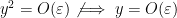
![\displaystyle V[R'] = \{ (y_1,\ldots,y_d) \in \tilde R^d: P_1(y_1,\ldots,y_d), \ldots, P_m(y_1,\ldots,y_d) = O(\varepsilon) \}](https://s0.wp.com/latex.php?latex=%5Cdisplaystyle++V%5BR%27%5D+%3D+%5C%7B+%28y_1%2C%5Cldots%2Cy_d%29+%5Cin+%5Ctilde+R%5Ed%3A+P_1%28y_1%2C%5Cldots%2Cy_d%29%2C+%5Cldots%2C+P_m%28y_1%2C%5Cldots%2Cy_d%29+%3D+O%28%5Cvarepsilon%29+%5C%7D+&bg=ffffff&fg=000000&s=0&c=20201002)

Thus we see that ![{V[{\bf R}]}](https://s0.wp.com/latex.php?latex=%7BV%5B%7B%5Cbf+R%7D%5D%7D&bg=ffffff&fg=000000&s=0&c=20201002)

![\displaystyle V_{(x)}[R'] = \{ y \in \tilde R: y = O(\varepsilon) \} \hbox{ mod } I,](https://s0.wp.com/latex.php?latex=%5Cdisplaystyle++V_%7B%28x%29%7D%5BR%27%5D+%3D+%5C%7B+y+%5Cin+%5Ctilde+R%3A+y+%3D+O%28%5Cvarepsilon%29+%5C%7D+%5Chbox%7B+mod+%7D+I%2C&bg=ffffff&fg=000000&s=0&c=20201002)
but the scheme associated to the smaller ideal 

![\displaystyle V_{(x^2)}[R'] = \{ y \in \tilde R: y^2 = O(\varepsilon) \} \hbox{ mod } I](https://s0.wp.com/latex.php?latex=%5Cdisplaystyle++V_%7B%28x%5E2%29%7D%5BR%27%5D+%3D+%5C%7B+y+%5Cin+%5Ctilde+R%3A+y%5E2+%3D+O%28%5Cvarepsilon%29+%5C%7D+%5Chbox%7B+mod+%7D+I&bg=ffffff&fg=000000&s=0&c=20201002)

Once one introduces the analyst’s epsilon, one can see quite clearly that ![{V_{(x^2)}[R']}](https://s0.wp.com/latex.php?latex=%7BV_%7B%28x%5E2%29%7D%5BR%27%5D%7D&bg=ffffff&fg=000000&s=0&c=20201002)
![{V_{(x)}[R']}](https://s0.wp.com/latex.php?latex=%7BV_%7B%28x%29%7D%5BR%27%5D%7D&bg=ffffff&fg=000000&s=0&c=20201002)
By working with this analyst’s extension of 
![\displaystyle V_{(x^2,y^2)}[R'] = \{ (x,y) \in \tilde R^2: x^2, y^2 = O(\varepsilon) \} \hbox{ mod } I^2](https://s0.wp.com/latex.php?latex=%5Cdisplaystyle++V_%7B%28x%5E2%2Cy%5E2%29%7D%5BR%27%5D+%3D+%5C%7B+%28x%2Cy%29+%5Cin+%5Ctilde+R%5E2%3A+x%5E2%2C+y%5E2+%3D+O%28%5Cvarepsilon%29+%5C%7D+%5Chbox%7B+mod+%7D+I%5E2+&bg=ffffff&fg=000000&s=0&c=20201002)

Note that the polynomial 

![{V_{(x^2,y^2)}[R'] = V_{(x^2,y^2,xy)}[R']}](https://s0.wp.com/latex.php?latex=%7BV_%7B%28x%5E2%2Cy%5E2%29%7D%5BR%27%5D+%3D+V_%7B%28x%5E2%2Cy%5E2%2Cxy%29%7D%5BR%27%5D%7D&bg=ffffff&fg=000000&s=0&c=20201002)


One can also view ideals (and hence, schemes), from a model-theoretic perspective. Let 

(since

for any assignment of indeterminates 

for all
we no longer have a counterexample to the converse coming from

so the extension
I have blogged a number of times in the past about the relationship between finitary (or “hard”, or “quantitative”) analysis, and infinitary (or “soft”, or “qualitative”) analysis. One way to connect the two types of analysis is via compactness arguments (and more specifically, contradiction and compactness arguments); such arguments can convert qualitative properties (such as continuity) to quantitative properties (such as bounded), basically because of the fundamental fact that continuous functions on a compact space are bounded (or the closely related fact that sequentially continuous functions on a sequentially compact space are bounded).
A key stage in any such compactness argument is the following: one has a sequence 
However, there is a slightly different approach, which I will call ultralimit analysis, which proceeds via the machinery of ultrafilters and ultraproducts; typically, the limit objects 

Ultralimit analysis is very closely related to nonstandard analysis. I already discussed some aspects of this relationship in an earlier post, and will expand upon it at the bottom of this post. Roughly speaking, the relationship between ultralimit analysis and nonstandard analysis is analogous to the relationship between measure theory and probability theory.
To illustrate how ultralimit analysis is actually used in practice, I will show later in this post how to take a qualitative infinitary theory – in this case, basic algebraic geometry – and apply ultralimit analysis to then deduce a quantitative version of this theory, in which the complexity of the various algebraic sets and varieties that appear as outputs are controlled uniformly by the complexity of the inputs. The point of this exercise is to show how ultralimit analysis allows for a relatively painless conversion back and forth between the quantitative and qualitative worlds, though in some cases the quantitative translation of a qualitative result (or vice versa) may be somewhat unexpected. In an upcoming paper of myself, Ben Green, and Emmanuel Breuillard (announced in the previous blog post), we will rely on ultralimit analysis to reduce the messiness of various quantitative arguments by replacing them with a qualitative setting in which the theory becomes significantly cleaner.
For sake of completeness, I also redo some earlier instances of the correspondence principle via ultralimit analysis, namely the deduction of the quantitative Gromov theorem from the qualitative one, and of Szemerédi’s theorem from the Furstenberg recurrence theorem, to illustrate how close the two techniques are to each other.

Recent Comments