You are currently browsing the tag archive for the ‘differential forms’ tag.

These lecture notes are a continuation of the 254A lecture notes from the previous quarter.
We consider the Euler equations for incompressible fluid flow on a Euclidean space {{\bf R}^d}; we will label {{\bf R}^d} as the “Eulerian space” {{\bf R}^d_E} (or “Euclidean space”, or “physical space”) to distinguish it from the “Lagrangian space” {{\bf R}^d_L} (or “labels space”) that we will introduce shortly (but the reader is free to also ignore the {E} or {L} subscripts if he or she wishes). Elements of Eulerian space {{\bf R}^d_E} will be referred to by symbols such as {x}, we use {dx} to denote Lebesgue measure on {{\bf R}^d_E} and we will use {x^1,\dots,x^d} for the {d} coordinates of {x}, and use indices such as {i,j,k} to index these coordinates (with the usual summation conventions), for instance {\partial_i} denotes partial differentiation along the {x^i} coordinate. (We use superscripts for coordinates {x^i} instead of subscripts {x_i} to be compatible with some differential geometry notation that we will use shortly; in particular, when using the summation notation, we will now be matching subscripts with superscripts for the pair of indices being summed.)
In Eulerian coordinates, the Euler equations read

\displaystyle  \partial_t u + u \cdot \nabla u = - \nabla p \ \ \ \ \ (1)

\displaystyle  \nabla \cdot u = 0

where {u: [0,T) \times {\bf R}^d_E \rightarrow {\bf R}^d_E} is the velocity field and {p: [0,T) \times {\bf R}^d_E \rightarrow {\bf R}} is the pressure field. These are functions of time {t \in [0,T)} and on the spatial location variable {x \in {\bf R}^d_E}. We will refer to the coordinates {(t,x) = (t,x^1,\dots,x^d)} as Eulerian coordinates. However, if one reviews the physical derivation of the Euler equations from 254A Notes 0, before one takes the continuum limit, the fundamental unknowns were not the velocity field {u} or the pressure field {p}, but rather the trajectories {(x^{(a)}(t))_{a \in A}}, which can be thought of as a single function {x: [0,T) \times A \rightarrow {\bf R}^d_E} from the coordinates {(t,a)} (where {t} is a time and {a} is an element of the label set {A}) to {{\bf R}^d}. The relationship between the trajectories {x^{(a)}(t) = x(t,a)} and the velocity field was given by the informal relationship

\displaystyle  \partial_t x(t,a) \approx u( t, x(t,a) ). \ \ \ \ \ (2)

We will refer to the coordinates {(t,a)} as (discrete) Lagrangian coordinates for describing the fluid.
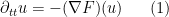
In view of this, it is natural to ask whether there is an alternate way to formulate the continuum limit of incompressible inviscid fluids, by using a continuous version {(t,a)} of the Lagrangian coordinates, rather than Eulerian coordinates. This is indeed the case. Suppose for instance one has a smooth solution {u, p} to the Euler equations on a spacetime slab {[0,T) \times {\bf R}^d_E} in Eulerian coordinates; assume furthermore that the velocity field {u} is uniformly bounded. We introduce another copy {{\bf R}^d_L} of {{\bf R}^d}, which we call Lagrangian space or labels space; we use symbols such as {a} to refer to elements of this space, {da} to denote Lebesgue measure on {{\bf R}^d_L}, and {a^1,\dots,a^d} to refer to the {d} coordinates of {a}. We use indices such as {\alpha,\beta,\gamma} to index these coordinates, thus for instance {\partial_\alpha} denotes partial differentiation along the {a^\alpha} coordinate. We will use summation conventions for both the Eulerian coordinates {i,j,k} and the Lagrangian coordinates {\alpha,\beta,\gamma}, with an index being summed if it appears as both a subscript and a superscript in the same term. While {{\bf R}^d_L} and {{\bf R}^d_E} are of course isomorphic, we will try to refrain from identifying them, except perhaps at the initial time {t=0} in order to fix the initialisation of Lagrangian coordinates.
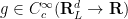
Given a smooth and bounded velocity field {u: [0,T) \times {\bf R}^d_E \rightarrow {\bf R}^d_E}, define a trajectory map for this velocity to be any smooth map {X: [0,T) \times {\bf R}^d_L \rightarrow {\bf R}^d_E} that obeys the ODE

\displaystyle  \partial_t X(t,a) = u( t, X(t,a) ); \ \ \ \ \ (3)

in view of (2), this describes the trajectory (in {{\bf R}^d_E}) of a particle labeled by an element {a} of {{\bf R}^d_L}. From the Picard existence theorem and the hypothesis that {u} is smooth and bounded, such a map exists and is unique as long as one specifies the initial location {X(0,a)} assigned to each label {a}. Traditionally, one chooses the initial condition

\displaystyle  X(0,a) = a \ \ \ \ \ (4)

for {a \in {\bf R}^d_L}, so that we label each particle by its initial location at time {t=0}; we are also free to specify other initial conditions for the trajectory map if we please. Indeed, we have the freedom to “permute” the labels {a \in {\bf R}^d_L} by an arbitrary diffeomorphism: if {X: [0,T) \times {\bf R}^d_L \rightarrow {\bf R}^d_E} is a trajectory map, and {\pi: {\bf R}^d_L \rightarrow{\bf R}^d_L} is any diffeomorphism (a smooth map whose inverse exists and is also smooth), then the map {X \circ \pi: [0,T) \times {\bf R}^d_L \rightarrow {\bf R}^d_E} is also a trajectory map, albeit one with different initial conditions {X(0,a)}.
Despite the popularity of the initial condition (4), we will try to keep conceptually separate the Eulerian space {{\bf R}^d_E} from the Lagrangian space {{\bf R}^d_L}, as they play different physical roles in the interpretation of the fluid; for instance, while the Euclidean metric {d\eta^2 = dx^1 dx^1 + \dots + dx^d dx^d} is an important feature of Eulerian space {{\bf R}^d_E}, it is not a geometrically natural structure to use in Lagrangian space {{\bf R}^d_L}. We have the following more general version of Exercise 8 from 254A Notes 2:

Exercise 1 Let {u: [0,T) \times {\bf R}^d_E \rightarrow {\bf R}^d_E} be smooth and bounded.

  • If {X_0: {\bf R}^d_L \rightarrow {\bf R}^d_E} is a smooth map, show that there exists a unique smooth trajectory map {X: [0,T) \times {\bf R}^d_L \rightarrow {\bf R}^d_E} with initial condition {X(0,a) = X_0(a)} for all {a \in {\bf R}^d_L}.
  • Show that if {X_0} is a diffeomorphism and {t \in [0,T)}, then the map {X(t): a \mapsto X(t,a)} is also a diffeomorphism.

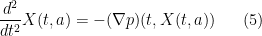
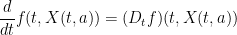
Remark 2 The first of the Euler equations (1) can now be written in the form

\displaystyle  \frac{d^2}{dt^2} X(t,a) = - (\nabla p)( t, X(t,a) ) \ \ \ \ \ (5)

which can be viewed as a continuous limit of Newton’s first law {m^{(a)} \frac{d^2}{dt^2} x^{(a)}(t) = F^{(a)}(t)}.

Call a diffeomorphism {Y: {\bf R}^d_L \rightarrow {\bf R}^d_E} (oriented) volume preserving if one has the equation

\displaystyle  \mathrm{det}( \nabla Y )(a) = 1 \ \ \ \ \ (6)

for all {a \in {\bf R}^d_L}, where the total differential {\nabla Y} is the {d \times d} matrix with entries {\partial_\alpha Y^i} for {\alpha = 1,\dots,d} and {i=1,\dots,d}, where {Y^1,\dots,Y^d:{\bf R}^d_L \rightarrow {\bf R}} are the components of {Y}. (If one wishes, one can also view {\nabla Y} as a linear transformation from the tangent space {T_a {\bf R}^d_L} of Lagrangian space at {a} to the tangent space {T_{Y(a)} {\bf R}^d_E} of Eulerian space at {Y(a)}.) Equivalently, {Y} is orientation preserving and one has a Jacobian-free change of variables formula

\displaystyle  \int_{{\bf R}^d_F} f( Y(a) )\ da = \int_{{\bf R}^d_E} f(x)\ dx

for all {f \in C_c({\bf R}^d_E \rightarrow {\bf R})}, which is in turn equivalent to {Y(E) \subset {\bf R}^d_E} having the same Lebesgue measure as {E} for any measurable set {E \subset {\bf R}^d_L}.
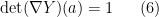
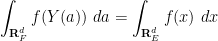
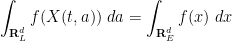
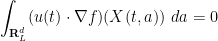
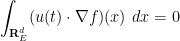
The divergence-free condition {\nabla \cdot u = 0} then can be nicely expressed in terms of volume-preserving properties of the trajectory maps {X}, in a manner which confirms the interpretation of this condition as an incompressibility condition on the fluid:

Lemma 3 Let {u: [0,T) \times {\bf R}^d_E \rightarrow {\bf R}^d_E} be smooth and bounded, let {X_0: {\bf R}^d_L \rightarrow {\bf R}^d_E} be a volume-preserving diffeomorphism, and let {X: [0,T) \times {\bf R}^d_L \rightarrow {\bf R}^d_E} be the trajectory map. Then the following are equivalent:

  • {\nabla \cdot u = 0} on {[0,T) \times {\bf R}^d_E}.
  • {X(t): {\bf R}^d_L \rightarrow {\bf R}^d_E} is volume-preserving for all
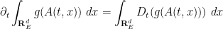
 {t \in [0,T)}.

Proof: Since {X_0} is orientation-preserving, we see from continuity that {X(t)} is also orientation-preserving. Suppose that {X(t)} is also volume-preserving, then for any {f \in C^\infty_c({\bf R}^d_E \rightarrow {\bf R})} we have the conservation law

\displaystyle  \int_{{\bf R}^d_L} f( X(t,a) )\ da = \int_{{\bf R}^d_E} f(x)\ dx

for all {t \in [0,T)}. Differentiating in time using the chain rule and (3) we conclude that

\displaystyle  \int_{{\bf R}^d_L} (u(t) \cdot \nabla f)( X(t,a)) \ da = 0

for all {t \in [0,T)}, and hence by change of variables

\displaystyle  \int_{{\bf R}^d_E} (u(t) \cdot \nabla f)(x) \ dx = 0

which by integration by parts gives

\displaystyle  \int_{{\bf R}^d_E} (\nabla \cdot u(t,x)) f(x)\ dx = 0

for all {f \in C^\infty_c({\bf R}^d_E \rightarrow {\bf R})} and {t \in [0,T)}, so {u} is divergence-free.
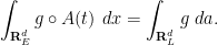
To prove the converse implication, it is convenient to introduce the labels map {A:[0,T) \times {\bf R}^d_E \rightarrow {\bf R}^d_L}, defined by setting {A(t): {\bf R}^d_E \rightarrow {\bf R}^d_L} to be the inverse of the diffeomorphism {X(t): {\bf R}^d_L \rightarrow {\bf R}^d_E}, thus

\displaystyle A(t, X(t,a)) = a

for all {(t,a) \in [0,T) \times {\bf R}^d_L}. By the implicit function theorem, {A} is smooth, and by differentiating the above equation in time using (3) we see that

\displaystyle  D_t A(t,x) = 0

where {D_t} is the usual material derivative

\displaystyle  D_t := \partial_t + u \cdot \nabla \ \ \ \ \ (7)

acting on functions on {[0,T) \times {\bf R}^d_E}. If {u} is divergence-free, we have from integration by parts that

\displaystyle  \partial_t \int_{{\bf R}^d_E} \phi(t,x)\ dx = \int_{{\bf R}^d_E} D_t \phi(t,x)\ dx

for any test function {\phi: [0,T) \times {\bf R}^d_E \rightarrow {\bf R}}. In particular, for any {g \in C^\infty_c({\bf R}^d_L \rightarrow {\bf R})}, we can calculate

\displaystyle \partial_t \int_{{\bf R}^d_E} g( A(t,x) )\ dx = \int_{{\bf R}^d_E} D_t (g(A(t,x)))\ dx

\displaystyle  = \int_{{\bf R}^d_E} 0\ dx

and hence

\displaystyle  \int_{{\bf R}^d_E} g(A(t,x))\ dx = \int_{{\bf R}^d_E} g(A(0,x))\ dx

for any {t \in [0,T)}. Since {X_0} is volume-preserving, so is {A(0)}, thus

\displaystyle  \int_{{\bf R}^d_E} g \circ A(t)\ dx = \int_{{\bf R}^d_L} g\ da.

Thus {A(t)} is volume-preserving, and hence {X(t)} is also. \Box

Exercise 4 Let {M: [0,T) \rightarrow \mathrm{GL}_d({\bf R})} be a continuously differentiable map from the time interval {[0,T)} to the general linear group {\mathrm{GL}_d({\bf R})} of invertible {d \times d} matrices. Establish Jacobi’s formula

\displaystyle  \partial_t \det(M(t)) = \det(M(t)) \mathrm{tr}( M(t)^{-1} \partial_t M(t) )

and use this and (6) to give an alternate proof of Lemma 3 that does not involve any integration in space.

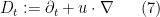
Remark 5 One can view the use of Lagrangian coordinates as an extension of the method of characteristics. Indeed, from the chain rule we see that for any smooth function {f: [0,T) \times {\bf R}^d_E \rightarrow {\bf R}} of Eulerian spacetime, one has

\displaystyle  \frac{d}{dt} f(t,X(t,a)) = (D_t f)(t,X(t,a))

and hence any transport equation that in Eulerian coordinates takes the form

\displaystyle  D_t f = g

for smooth functions {f,g: [0,T) \times {\bf R}^d_E \rightarrow {\bf R}} of Eulerian spacetime is equivalent to the ODE

\displaystyle  \frac{d}{dt} F = G

where {F,G: [0,T) \times {\bf R}^d_L \rightarrow {\bf R}} are the smooth functions of Lagrangian spacetime defined by

\displaystyle  F(t,a) := f(t,X(t,a)); \quad G(t,a) := g(t,X(t,a)).

In this set of notes we recall some basic differential geometry notation, particularly with regards to pullbacks and Lie derivatives of differential forms and other tensor fields on manifolds such as {{\bf R}^d_E} and {{\bf R}^d_L}, and explore how the Euler equations look in this notation. Our discussion will be entirely formal in nature; we will assume that all functions have enough smoothness and decay at infinity to justify the relevant calculations. (It is possible to work rigorously in Lagrangian coordinates – see for instance the work of Ebin and Marsden – but we will not do so here.) As a general rule, Lagrangian coordinates tend to be somewhat less convenient to use than Eulerian coordinates for establishing the basic analytic properties of the Euler equations, such as local existence, uniqueness, and continuous dependence on the data; however, they are quite good at clarifying the more algebraic properties of these equations, such as conservation laws and the variational nature of the equations. It may well be that in the future we will be able to use the Lagrangian formalism more effectively on the analytic side of the subject also.

Remark 6 One can also write the Navier-Stokes equations in Lagrangian coordinates, but the equations are not expressed in a favourable form in these coordinates, as the Laplacian {\Delta} appearing in the viscosity term becomes replaced with a time-varying Laplace-Beltrami operator. As such, we will not discuss the Lagrangian coordinate formulation of Navier-Stokes here.

Read the rest of this entry »

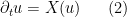
I’ve just uploaded to the arXiv my paper “On the universality of potential well dynamics“, submitted to Dynamics of PDE. This is a spinoff from my previous paper on blowup of nonlinear wave equations, inspired by some conversations with Sungjin Oh. Here we focus mainly on the zero-dimensional case of such equations, namely the potential well equation

\displaystyle  \partial_{tt} u = - (\nabla F)(u) \ \ \ \ \ (1)

for a particle {u: {\bf R} \rightarrow {\bf R}^m} trapped in a potential well with potential {F: {\bf R}^m \rightarrow {\bf R}}, with {F(z) \rightarrow +\infty} as {z \rightarrow \infty}. This ODE always admits global solutions from arbitrary initial positions {u(0)} and initial velocities {\partial_t u(0)}, thanks to conservation of the Hamiltonian {\frac{1}{2} |\partial_t u|^2 + F(u)}. As this Hamiltonian is coercive (in that its level sets are compact), solutions to this equation are always almost periodic. On the other hand, as can already be seen using the harmonic oscillator {\partial_{tt} u = - k^2 u} (and direct sums of this system), this equation can generate periodic solutions, as well as quasiperiodic solutions.

All quasiperiodic motions are almost periodic. However, there are many examples of dynamical systems that admit solutions that are almost periodic but not quasiperiodic. So one can pose the question: are the dynamics of potential wells universal in the sense that they can capture all almost periodic solutions?

A precise question can be phrased as follows. Let {M} be a compact manifold, and let {X} be a smooth vector field on {M}; to avoid degeneracies, let us take {X} to be non-singular in the sense that it is everywhere non-vanishing. Then the trajectories of the first-order ODE

\displaystyle  \partial_t u = X(u) \ \ \ \ \ (2)

for {u: {\bf R} \rightarrow M} are always global and almost periodic. Can we then find a (coercive) potential {F: {\bf R}^m \rightarrow {\bf R}} for some {m}, as well as a smooth embedding {\phi: M \rightarrow {\bf R}^m}, such that every solution {u} to (2) pushes forward under {\phi} to a solution to (1)? (Actually, for technical reasons it is preferable to map into the phase space {{\bf R}^m \times {\bf R}^m}, rather than position space {{\bf R}^m}, but let us ignore this detail for this discussion.)

It turns out that the answer is no; there is a very specific obstruction. Given a pair {(M,X)} as above, define a strongly adapted {1}-form to be a {1}-form {\phi} on {M} such that {\phi(X)} is pointwise positive, and the Lie derivative {{\mathcal L}_X \phi} is an exact {1}-form. We then have

Theorem 1 A smooth compact non-singular dynamics {(M,X)} can be embedded smoothly in a potential well system if and only if it admits a strongly adapted {1}-form.

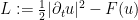
For the “only if” direction, the key point is that potential wells (viewed as a Hamiltonian flow on the phase space {{\bf R}^m \times {\bf R}^m}) admit a strongly adapted {1}-form, namely the canonical {1}-form {p dq}, whose Lie derivative is the derivative {dL} of the Lagrangian {L := \frac{1}{2} |\partial_t u|^2 - F(u)} and is thus exact. The converse “if” direction is mainly a consequence of the Nash embedding theorem, and follows the arguments used in my previous paper.

Interestingly, the same obstruction also works for potential wells in a more general Riemannian manifold than {{\bf R}^m}, or for nonlinear wave equations with a potential; combining the two, the obstruction is also present for wave maps with a potential.

It is then natural to ask whether this obstruction is non-trivial, in the sense that there are at least some examples of dynamics {(M,X)} that do not support strongly adapted {1}-forms (and hence cannot be modeled smoothly by the dynamics of a potential well, nonlinear wave equation, or wave maps). I posed this question on MathOverflow, and Robert Bryant provided a very nice construction, showing that the vector field {(\sin(2\pi x), \cos(2\pi x))} on the {2}-torus {({\bf R}/{\bf Z})^2} had no strongly adapted {1}-forms, and hence the dynamics of this vector field cannot be smoothly reproduced by a potential well, nonlinear wave equation, or wave map:

On the other hand, the suspension of any diffeomorphism does support a strongly adapted {1}-form (the derivative {dt} of the time coordinate), and using this and the previous theorem I was able to embed a universal Turing machine into a potential well. In particular, there are flows for an explicitly describable potential well whose trajectories have behavior that is undecidable using the usual ZFC axioms of set theory! So potential well dynamics are “effectively” universal, despite the presence of the aforementioned obstruction.

In my previous work on blowup for Navier-Stokes like equations, I speculated that if one could somehow replicate a universal Turing machine within the Euler equations, one could use this machine to create a “von Neumann machine” that replicated smaller versions of itself, which on iteration would lead to a finite time blowup. Now that such a mechanism is present in nonlinear wave equations, it is tempting to try to make this scheme work in that setting. Of course, in my previous paper I had already demonstrated finite time blowup, at least in a three-dimensional setting, but that was a relatively simple discretely self-similar blowup in which no computation occurred. This more complicated blowup scheme would be significantly more effort to set up, but would be proof-of-concept that the same scheme would in principle be possible for the Navier-Stokes equations, assuming somehow that one can embed a universal Turing machine into the Euler equations. (But I’m still hopelessly stuck on how to accomplish this latter task…)

In 1946, Ulam, in response to a theorem of Anning and Erdös, posed the following problem:

Problem 1 (Erdös-Ulam problem) Let {S \subset {\bf R}^2} be a set such that the distance between any two points in {S} is rational. Is it true that {S} cannot be (topologically) dense in {{\bf R}^2}?

The paper of Anning and Erdös addressed the case that all the distances between two points in {S} were integer rather than rational in the affirmative.

The Erdös-Ulam problem remains open; it was discussed recently over at Gödel’s lost letter. It is in fact likely (as we shall see below) that the set {S} in the above problem is not only forbidden to be topologically dense, but also cannot be Zariski dense either. If so, then the structure of {S} is quite restricted; it was shown by Solymosi and de Zeeuw that if {S} fails to be Zariski dense, then all but finitely many of the points of {S} must lie on a single line, or a single circle. (Conversely, it is easy to construct examples of dense subsets of a line or circle in which all distances are rational, though in the latter case the square of the radius of the circle must also be rational.)

The main tool of the Solymosi-de Zeeuw analysis was Faltings’ celebrated theorem that every algebraic curve of genus at least two contains only finitely many rational points. The purpose of this post is to observe that an affirmative answer to the full Erdös-Ulam problem similarly follows from the conjectured analogue of Falting’s theorem for surfaces, namely the following conjecture of Bombieri and Lang:

Conjecture 2 (Bombieri-Lang conjecture) Let {X} be a smooth projective irreducible algebraic surface defined over the rationals {{\bf Q}} which is of general type. Then the set {X({\bf Q})} of rational points of {X} is not Zariski dense in {X}.

In fact, the Bombieri-Lang conjecture has been made for varieties of arbitrary dimension, and for more general number fields than the rationals, but the above special case of the conjecture is the only one needed for this application. We will review what “general type” means (for smooth projective complex varieties, at least) below the fold.

The Bombieri-Lang conjecture is considered to be extremely difficult, in particular being substantially harder than Faltings’ theorem, which is itself a highly non-trivial result. So this implication should not be viewed as a practical route to resolving the Erdös-Ulam problem unconditionally; rather, it is a demonstration of the power of the Bombieri-Lang conjecture. Still, it was an instructive algebraic geometry exercise for me to carry out the details of this implication, which quickly boils down to verifying that a certain quite explicit algebraic surface is of general type (Theorem 4 below). As I am not an expert in the subject, my computations here will be rather tedious and pedestrian; it is likely that they could be made much slicker by exploiting more of the machinery of modern algebraic geometry, and I would welcome any such streamlining by actual experts in this area. (For similar reasons, there may be more typos and errors than usual in this post; corrections are welcome as always.) My calculations here are based on a similar calculation of van Luijk, who used analogous arguments to show (assuming Bombieri-Lang) that the set of perfect cuboids is not Zariski-dense in its projective parameter space.

We also remark that in a recent paper of Makhul and Shaffaf, the Bombieri-Lang conjecture (or more precisely, a weaker consequence of that conjecture) was used to show that if {S} is a subset of {{\bf R}^2} with rational distances which intersects any line in only finitely many points, then there is a uniform bound on the cardinality of the intersection of {S} with any line. I have also recently learned (private communication) that an unpublished work of Shaffaf has obtained a result similar to the one in this post, namely that the Erdös-Ulam conjecture follows from the Bombieri-Lang conjecture, plus an additional conjecture about the rational curves in a specific surface.

Let us now give the elementary reductions to the claim that a certain variety is of general type. For sake of contradiction, let {S} be a dense set such that the distance between any two points is rational. Then {S} certainly contains two points that are a rational distance apart. By applying a translation, rotation, and a (rational) dilation, we may assume that these two points are {(0,0)} and {(1,0)}. As {S} is dense, there is a third point of {S} not on the {x} axis, which after a reflection we can place in the upper half-plane; we will write it as {(a,\sqrt{b})} with {b>0}.

Given any two points {P, Q} in {S}, the quantities {|P|^2, |Q|^2, |P-Q|^2} are rational, and so by the cosine rule the dot product {P \cdot Q} is rational as well. Since {(1,0) \in S}, this implies that the {x}-component of every point {P} in {S} is rational; this in turn implies that the product of the {y}-coordinates of any two points {P,Q} in {S} is rational as well (since this differs from {P \cdot Q} by a rational number). In particular, {a} and {b} are rational, and all of the points in {S} now lie in the lattice {\{ ( x, y\sqrt{b}): x, y \in {\bf Q} \}}. (This fact appears to have first been observed in the 1988 habilitationschrift of Kemnitz.)

Now take four points {(x_j,y_j \sqrt{b})}, {j=1,\dots,4} in {S} in general position (so that the octuplet {(x_1,y_1\sqrt{b},\dots,x_4,y_4\sqrt{b})} avoids any pre-specified hypersurface in {{\bf C}^8}); this can be done if {S} is dense. (If one wished, one could re-use the three previous points {(0,0), (1,0), (a,\sqrt{b})} to be three of these four points, although this ultimately makes little difference to the analysis.) If {(x,y\sqrt{b})} is any point in {S}, then the distances {r_j} from {(x,y\sqrt{b})} to {(x_j,y_j\sqrt{b})} are rationals that obey the equations

\displaystyle (x - x_j)^2 + b (y-y_j)^2 = r_j^2

for {j=1,\dots,4}, and thus determine a rational point in the affine complex variety {V = V_{b,x_1,y_1,x_2,y_2,x_3,y_3,x_4,y_4} \subset {\bf C}^5} defined as

\displaystyle V := \{ (x,y,r_1,r_2,r_3,r_4) \in {\bf C}^6:

\displaystyle (x - x_j)^2 + b (y-y_j)^2 = r_j^2 \hbox{ for } j=1,\dots,4 \}.

By inspecting the projection {(x,y,r_1,r_2,r_3,r_4) \rightarrow (x,y)} from {V} to {{\bf C}^2}, we see that {V} is a branched cover of {{\bf C}^2}, with the generic cover having {2^4=16} points (coming from the different ways to form the square roots {r_1,r_2,r_3,r_4}); in particular, {V} is a complex affine algebraic surface, defined over the rationals. By inspecting the monodromy around the four singular base points {(x,y) = (x_i,y_i)} (which switch the sign of one of the roots {r_i}, while keeping the other three roots unchanged), we see that the variety {V} is connected away from its singular set, and thus irreducible. As {S} is topologically dense in {{\bf R}^2}, it is Zariski-dense in {{\bf C}^2}, and so {S} generates a Zariski-dense set of rational points in {V}. To solve the Erdös-Ulam problem, it thus suffices to show that

Claim 3 For any non-zero rational {b} and for rationals {x_1,y_1,x_2,y_2,x_3,y_3,x_4,y_4} in general position, the rational points of the affine surface {V = V_{b,x_1,y_1,x_2,y_2,x_3,y_3,x_4,y_4}} is not Zariski dense in {V}.

This is already very close to a claim that can be directly resolved by the Bombieri-Lang conjecture, but {V} is affine rather than projective, and also contains some singularities. The first issue is easy to deal with, by working with the projectivisation

\displaystyle \overline{V} := \{ [X,Y,Z,R_1,R_2,R_3,R_4] \in {\bf CP}^6: Q(X,Y,Z,R_1,R_2,R_3,R_4) = 0 \} \ \ \ \ \ (1)


of {V}, where {Q: {\bf C}^7 \rightarrow {\bf C}^4} is the homogeneous quadratic polynomial

\displaystyle (X,Y,Z,R_1,R_2,R_3,R_4) := (Q_j(X,Y,Z,R_1,R_2,R_3,R_4) )_{j=1}^4

with

\displaystyle Q_j(X,Y,Z,R_1,R_2,R_3,R_4) := (X-x_j Z)^2 + b (Y-y_jZ)^2 - R_j^2

and the projective complex space {{\bf CP}^6} is the space of all equivalence classes {[X,Y,Z,R_1,R_2,R_3,R_4]} of tuples {(X,Y,Z,R_1,R_2,R_3,R_4) \in {\bf C}^7 \backslash \{0\}} up to projective equivalence {(\lambda X, \lambda Y, \lambda Z, \lambda R_1, \lambda R_2, \lambda R_3, \lambda R_4) \sim (X,Y,Z,R_1,R_2,R_3,R_4)}. By identifying the affine point {(x,y,r_1,r_2,r_3,r_4)} with the projective point {(X,Y,1,R_1,R_2,R_3,R_4)}, we see that {\overline{V}} consists of the affine variety {V} together with the set {\{ [X,Y,0,R_1,R_2,R_3,R_4]: X^2+bY^2=R^2; R_j = \pm R_1 \hbox{ for } j=2,3,4\}}, which is the union of eight curves, each of which lies in the closure of {V}. Thus {\overline{V}} is the projective closure of {V}, and is thus a complex irreducible projective surface, defined over the rationals. As {\overline{V}} is cut out by four quadric equations in {{\bf CP}^6} and has degree sixteen (as can be seen for instance by inspecting the intersection of {\overline{V}} with a generic perturbation of a fibre over the generically defined projection {[X,Y,Z,R_1,R_2,R_3,R_4] \mapsto [X,Y,Z]}), it is also a complete intersection. To show (3), it then suffices to show that the rational points in {\overline{V}} are not Zariski dense in {\overline{V}}.

Heuristically, the reason why we expect few rational points in {\overline{V}} is as follows. First observe from the projective nature of (1) that every rational point is equivalent to an integer point. But for a septuple {(X,Y,Z,R_1,R_2,R_3,R_4)} of integers of size {O(N)}, the quantity {Q(X,Y,Z,R_1,R_2,R_3,R_4)} is an integer point of {{\bf Z}^4} of size {O(N^2)}, and so should only vanish about {O(N^{-8})} of the time. Hence the number of integer points {(X,Y,Z,R_1,R_2,R_3,R_4) \in {\bf Z}^7} of height comparable to {N} should be about

\displaystyle O(N)^7 \times O(N^{-8}) = O(N^{-1});

this is a convergent sum if {N} ranges over (say) powers of two, and so from standard probabilistic heuristics (see this previous post) we in fact expect only finitely many solutions, in the absence of any special algebraic structure (e.g. the structure of an abelian variety, or a birational reduction to a simpler variety) that could produce an unusually large number of solutions.

The Bombieri-Lang conjecture, Conjecture 2, can be viewed as a formalisation of the above heuristics (roughly speaking, it is one of the most optimistic natural conjectures one could make that is compatible with these heuristics while also being invariant under birational equivalence).

Unfortunately, {\overline{V}} contains some singular points. Being a complete intersection, this occurs when the Jacobian matrix of the map {Q: {\bf C}^7 \rightarrow {\bf C}^4} has less than full rank, or equivalently that the gradient vectors

\displaystyle \nabla Q_j = (2(X-x_j Z), 2(Y-y_j Z), -2x_j (X-x_j Z) - 2y_j (Y-y_j Z), \ \ \ \ \ (2)


\displaystyle 0, \dots, 0, -2R_j, 0, \dots, 0)

for {j=1,\dots,4} are linearly dependent, where the {-2R_j} is in the coordinate position associated to {R_j}. One way in which this can occur is if one of the gradient vectors {\nabla Q_j} vanish identically. This occurs at precisely {4 \times 2^3 = 32} points, when {[X,Y,Z]} is equal to {[x_j,y_j,1]} for some {j=1,\dots,4}, and one has {R_k = \pm ( (x_j - x_k)^2 + b (y_j - y_k)^2 )^{1/2}} for all {k=1,\dots,4} (so in particular {R_j=0}). Let us refer to these as the obvious singularities; they arise from the geometrically evident fact that the distance function {(x,y\sqrt{b}) \mapsto \sqrt{(x-x_j)^2 + b(y-y_j)^2}} is singular at {(x_j,y_j\sqrt{b})}.

The other way in which could occur is if a non-trivial linear combination of at least two of the gradient vectors vanishes. From (2), this can only occur if {R_j=R_k=0} for some distinct {j,k}, which from (1) implies that

\displaystyle (X - x_j Z) = \pm \sqrt{b} i (Y - y_j Z) \ \ \ \ \ (3)


and

\displaystyle (X - x_k Z) = \pm \sqrt{b} i (Y - y_k Z) \ \ \ \ \ (4)


for two choices of sign {\pm}. If the signs are equal, then (as {x_j, y_j, x_k, y_k} are in general position) this implies that {Z=0}, and then we have the singular point

\displaystyle [X,Y,Z,R_1,R_2,R_3,R_4] = [\pm \sqrt{b} i, 1, 0, 0, 0, 0, 0]. \ \ \ \ \ (5)


If the non-trivial linear combination involved three or more gradient vectors, then by the pigeonhole principle at least two of the signs involved must be equal, and so the only singular points are (5). So the only remaining possibility is when we have two gradient vectors {\nabla Q_j, \nabla Q_k} that are parallel but non-zero, with the signs in (3), (4) opposing. But then (as {x_j,y_j,x_k,y_k} are in general position) the vectors {(X-x_j Z, Y-y_j Z), (X-x_k Z, Y-y_k Z)} are non-zero and non-parallel to each other, a contradiction. Thus, outside of the {32} obvious singular points mentioned earlier, the only other singular points are the two points (5).

We will shortly show that the {32} obvious singularities are ordinary double points; the surface {\overline{V}} near any of these points is analytically equivalent to an ordinary cone {\{ (x,y,z) \in {\bf C}^3: z^2 = x^2 + y^2 \}} near the origin, which is a cone over a smooth conic curve {\{ (x,y) \in {\bf C}^2: x^2+y^2=1\}}. The two non-obvious singularities (5) are slightly more complicated than ordinary double points, they are elliptic singularities, which approximately resemble a cone over an elliptic curve. (As far as I can tell, this resemblance is exact in the category of real smooth manifolds, but not in the category of algebraic varieties.) If one blows up each of the point singularities of {\overline{V}} separately, no further singularities are created, and one obtains a smooth projective surface {X} (using the Segre embedding as necessary to embed {X} back into projective space, rather than in a product of projective spaces). Away from the singularities, the rational points of {\overline{V}} lift up to rational points of {X}. Assuming the Bombieri-Lang conjecture, we thus are able to answer the Erdös-Ulam problem in the affirmative once we establish

Theorem 4 The blowup {X} of {\overline{V}} is of general type.

This will be done below the fold, by the pedestrian device of explicitly constructing global differential forms on {X}; I will also be working from a complex analysis viewpoint rather than an algebraic geometry viewpoint as I am more comfortable with the former approach. (As mentioned above, though, there may well be a quicker way to establish this result by using more sophisticated machinery.)

I thank Mark Green and David Gieseker for helpful conversations (and a crash course in varieties of general type!).

Remark 5 The above argument shows in fact (assuming Bombieri-Lang) that sets {S \subset {\bf R}^2} with all distances rational cannot be Zariski-dense, and thus (by Solymosi-de Zeeuw) must lie on a single line or circle with only finitely many exceptions. Assuming a stronger version of Bombieri-Lang involving a general number field {K}, we obtain a similar conclusion with “rational” replaced by “lying in {K}” (one has to extend the Solymosi-de Zeeuw analysis to more general number fields, but this should be routine, using the analogue of Faltings’ theorem for such number fields).

Read the rest of this entry »

I’m continuing my series of articles for the Princeton Companion to Mathematics through the holiday season with my article on “Differential forms and integration“. This is my attempt to explain the concept of a differential form in differential geometry and several variable calculus; which I view as an extension of the concept of the signed integral in single variable calculus. I briefly touch on the important concept of de Rham cohomology, but mostly I stick to fundamentals.

I would also like to highlight Doron Zeilberger‘s PCM article “Enumerative and Algebraic combinatorics“. This article describes the art of how to usefully count the number of objects of a given type exactly; this subject has a rather algebraic flavour to it, in contrast with asymptotic combinatorics, which is more concerned with computing the order of magnitude of number of objects in a class. The two subjects complement each other; for instance, in my own work, I have found enumerative and other algebraic methods tend to be useful for controlling “main terms” in a given expression, while asymptotic and other analytic methods tend to be good at controlling “error terms”.

Archives