The spectral proof of the Szemeredi regularity lemma

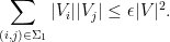
Perhaps the most important structural result about general large dense graphs is the Szemerédi regularity lemma. Here is a standard formulation of that lemma:

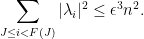
Lemma 1 (Szemerédi regularity lemma) Let be a graph on vertices, and let . Then there exists a partition for some with the property that for all but at most of the pairs , the pair is -regular in the sense that

whenever are such that and , and is the edge density between and . Furthermore, the partition is equitable in the sense that for all .

There are many proofs of this lemma, which is actually not that difficult to establish; see for instance these previous blog posts for some examples. In this post I would like to record one further proof, based on the spectral decomposition of the adjacency matrix of , which is essentially due to Frieze and Kannan. (Strictly speaking, Frieze and Kannan used a variant of this argument to establish a weaker form of the regularity lemma, but it is not difficult to modify the Frieze-Kannan argument to obtain the usual form of the regularity lemma instead. Some closely related spectral regularity lemmas were also developed by Szegedy.) I found recently (while speaking at the Abel conference in honour of this year’s laureate, Endre Szemerédi) that this particular argument is not as widely known among graph theory experts as I had thought, so I thought I would record it here.

For reasons of exposition, it is convenient to first establish a slightly weaker form of the lemma, in which one drops the hypothesis of equitability (but then has to weight the cells by their magnitude when counting bad pairs):

Lemma 2 (Szemerédi regularity lemma, weakened variant) . Let be a graph on vertices, and let . Then there exists a partition for some with the property that for all pairs outside of an exceptional set , one has

whenever , for some real number , where is the number of edges between and . Furthermore, we have

Let us now prove Lemma 2. We enumerate (after relabeling) as . The adjacency matrix of the graph is then a self-adjoint matrix, and thus admits an eigenvalue decomposition

for some orthonormal basis of and some eigenvalues , which we arrange in decreasing order of magnitude:

We can compute the trace of as

But we also have , so

Among other things, this implies that

for all .

Let be a function (depending on ) to be chosen later, with for all . Applying (3) and the pigeonhole principle (or the finite convergence principle, see this blog post), we can find such that

(Indeed, the bound on is basically iterated times.) We can now split

where is the “structured” component

is the “small” component

and is the “pseudorandom” component

We now design a vertex partition to make approximately constant on most cells. For each , we partition into cells on which (viewed as a function from to ) only fluctuates by , plus an exceptional cell of size coming from the values where is excessively large (larger than ). Combining all these partitions together, we can write for some , where has cardinality at most , and for all , the eigenfunctions all fluctuate by at most . In particular, if , then (by (4) and (6)) the entries of fluctuate by at most on each block . If we let be the mean value of these entries on , we thus have

for any and , where we view the indicator functions as column vectors of dimension .

Next, we observe from (3) and (7) that . If we let be the coefficients of , we thus have

and hence by Markov’s inequality we have

for all pairs outside of an exceptional set with

If avoids , we thus have

for any , by (10) and the Cauchy-Schwarz inequality.

Finally, to control we see from (4) and (8) that has an operator norm of at most . In particular, we have from the Cauchy-Schwarz inequality that

for any .

Let be the set of all pairs where either , , , or

One easily verifies that (2) holds. If is not in , then by summing (9), (11), (12) and using (5), we see that

for all . The left-hand side is just . As , we have

and so (since )

If we let be a sufficiently rapidly growing function of that depends on , the second error term in (13) can be absorbed in the first, and (1) follows. This concludes the proof of Lemma 2.

To prove Lemma 1, one argues similarly (after modifying as necessary), except that the initial partition of constructed above needs to be subdivided further into equitable components (of size ), plus some remainder sets which can be aggregated into an exceptional component of size (and which can then be redistributed amongst the other components to arrive at a truly equitable partition). We omit the details.

Remark 1 It is easy to verify that needs to be growing exponentially in in order for the above argument to work, which leads to tower-exponential bounds in the number of cells in the partition. It was shown by Gowers that a tower-exponential bound is actually necessary here. By varying , one basically obtains the strong regularity lemma first established by Alon, Fischer, Krivelevich, and Szegedy; in the opposite direction, setting essentially gives the weak regularity lemma of Frieze and Kannan.

Remark 2 If we specialise to a Cayley graph, in which is a finite abelian group and for some (symmetric) subset of , then the eigenvectors are characters, and one essentially recovers the arithmetic regularity lemma of Green, in which the vertex partition classes are given by Bohr sets (and one can then place additional regularity properties on these Bohr sets with some additional arguments). The components of , representing high, medium, and low eigenvalues of , then become a decomposition associated to high, medium, and low Fourier coefficients of .

Remark 3 The use of spectral theory here is parallel to the use of Fourier analysis to establish results such as Roth’s theorem on arithmetic progressions of length three. In analogy with this, one could view hypergraph regularity as being a sort of “higher order spectral theory”, although this spectral perspective is not as convenient as it is in the graph case.

Some ingredients in Szemerédi’s proof of Szemerédi’s theorem

A few days ago, Endre Szemerédi was awarded the 2012 Abel prize “for his fundamental contributions to discrete mathematics and theoretical computer science, and in recognition of the profound and lasting impact of these contributions on additive number theory and ergodic theory.” The full citation for the prize may be found here, and the written notes for a talk given by Tim Gowers on Endre’s work at the announcement may be found here (and video of the talk can be found here).

As I was on the Abel prize committee this year, I won’t comment further on the prize, but will instead focus on what is arguably Endre’s most well known result, namely Szemerédi’s theorem on arithmetic progressions:

Theorem 1 (Szemerédi’s theorem) Let be a set of integers of positive upper density, thus , where . Then contains an arithmetic progression of length for any .

Szemerédi’s original proof of this theorem is a remarkably intricate piece of combinatorial reasoning. Most proofs of theorems in mathematics – even long and difficult ones – generally come with a reasonably compact “high-level” overview, in which the proof is (conceptually, at least) broken down into simpler pieces. There may well be technical difficulties in formulating and then proving each of the component pieces, and then in fitting the pieces together, but usually the “big picture” is reasonably clear. To give just one example, the overall strategy of Perelman’s proof of the Poincaré conjecture can be briefly summarised as follows: to show that a simply connected three-dimensional manifold is homeomorphic to a sphere, place a Riemannian metric on it and perform Ricci flow, excising any singularities that arise by surgery, until the entire manifold becomes extinct. By reversing the flow and analysing the surgeries performed, obtain enough control on the topology of the original manifold to establish that it is a topological sphere.

In contrast, the pieces of Szemerédi’s proof are highly interlocking, particularly with regard to all the epsilon-type parameters involved; it takes quite a bit of notational setup and foundational lemmas before the key steps of the proof can even be stated, let alone proved. Szemerédi’s original paper contains a logical diagram of the proof (reproduced in Gowers’ recent talk) which already gives a fair indication of this interlocking structure. (Many years ago I tried to present the proof, but I was unable to find much of a simplification, and my exposition is probably not that much clearer than the original text.) Even the use of nonstandard analysis, which is often helpful in cleaning up armies of epsilons, turns out to be a bit tricky to apply here. (In typical applications of nonstandard analysis, one can get by with a single nonstandard universe, constructed as an ultrapower of the standard universe; but to correctly model all the epsilons occuring in Szemerédi’s argument, one needs to repeatedly perform the ultrapower construction to obtain a (finite) sequence of increasingly nonstandard (and increasingly saturated) universes, each one containing unbounded quantities that are far larger than any quantity that appears in the preceding universe, as discussed at the end of this previous blog post. This sequence of universes does end up concealing all the epsilons, but it is not so clear that this is a net gain in clarity for the proof; I may return to the nonstandard presentation of Szemeredi’s argument at some future juncture.)

Instead of trying to describe the entire argument here, I thought I would instead show some key components of it, with only the slightest hint as to how to assemble the components together to form the whole proof. In particular, I would like to show how two particular ingredients in the proof – namely van der Waerden’s theorem and the Szemerédi regularity lemma – become useful. For reasons that will hopefully become clearer later, it is convenient not only to work with ordinary progressions , but also progressions of progressions , progressions of progressions of progressions, and so forth. (In additive combinatorics, these objects are known as generalised arithmetic progressions of rank one, two, three, etc., and play a central role in the subject, although the way they are used in Szemerédi’s proof is somewhat different from the way that they are normally used in additive combinatorics.) Very roughly speaking, Szemerédi’s proof begins by building an enormous generalised arithmetic progression of high rank containing many elements of the set (arranged in a “near-maximal-density” configuration), and then steadily prunes this progression to improve the combinatorial properties of the configuration, until one ends up with a single rank one progression of length that consists entirely of elements of .

To illustrate some of the basic ideas, let us first consider a situation in which we have located a progression of progressions of length , with each progression , being quite long, and containing a near-maximal amount of elements of , thus

where is the “maximal density” of along arithmetic progressions. (There are a lot of subtleties in the argument about exactly how good the error terms are in various approximations, but we will ignore these issues for the sake of this discussion and just use the imprecise symbols such as instead.) By hypothesis, is positive. The objective is then to locate a progression in , with each in for . It may help to view the progression of progressions as a tall thin rectangle .

If we write for , then the problem is equivalent to finding a (possibly degenerate) arithmetic progression , with each in .

By hypothesis, we know already that each set has density about in :

Let us now make a “weakly mixing” assumption on the , which roughly speaking asserts that

for “most” subsets of of density of a certain form to be specified shortly. This is a plausible type of assumption if one believes to behave like a random set, and if the sets are constructed “independently” of the in some sense. Of course, we do not expect such an assumption to be valid all of the time, but we will postpone consideration of this point until later. Let us now see how this sort of weakly mixing hypothesis could help one count progressions of the desired form.

We will inductively consider the following (nonrigorously defined) sequence of claims for each :

• : For most choices of , there are arithmetic progressions in with the specified choice of , such that for all .

(Actually, to avoid boundary issues one should restrict to lie in the middle third of , rather than near the edges, but let us ignore this minor technical detail.) The quantity is natural here, given that there are arithmetic progressions in that pass through in the position, and that each one ought to have a probability of or so that the events simultaneously hold.) If one has the claim , then by selecting a typical in , we obtain a progression with for all , as required. (In fact, we obtain about such progressions by this method.)

We can heuristically justify the claims by induction on . For , the claims are clear just from direct counting of progressions (as long as we keep away from the edges of ). Now suppose that , and the claims have already been proven. For any and for most , we have from hypothesis that there are progressions in through with . Let be the set of all the values of attained by these progressions, then . Invoking the weak mixing hypothesis, we (heuristically, at least) conclude that for most choices of , we have

which then gives the desired claim .

The observant reader will note that we only needed the claim in the case for the above argument, but for technical reasons, the full proof requires one to work with more general values of (also the claim needs to be replaced by a more complicated version of itself, but let’s ignore this for sake of discussion).

We now return to the question of how to justify the weak mixing hypothesis (2). For a single block of , one can easily concoct a scenario in which this hypothesis fails, by choosing to overlap with too strongly, or to be too disjoint from . However, one can do better if one can select from a long progression of blocks. The starting point is the following simple double counting observation that gives the right upper bound:

Proposition 2 (Single upper bound) Let be a progression of progressions for some large . Suppose that for each , the set has density in (i.e. (1) holds). Let be a subset of of density . Then (if is large enough) one can find an such that

Proof: The key is the double counting identity

Because has maximal density and is large, we have

for each , and thus

The claim then follows from the pigeonhole principle.

Now suppose we want to obtain weak mixing not just for a single set , but for a small number of such sets, i.e. we wish to find an for which

for all , where is the density of in . The above proposition gives, for each , a choice of for which (3) holds, but it could be a different for each , and so it is not immediately obvious how to use Proposition 2 to find an for which (3) holds simultaneously for all . However, it turns out that the van der Waerden theorem is the perfect tool for this amplification:

Proposition 3 (Multiple upper bound) Let be a progression of progressions for some large . Suppose that for each , the set has density in (i.e. (1) holds). For each , let be a subset of of density . Then (if is large enough depending on ) one can find an such that

simultaneously for all .

Proof: Suppose that the claim failed (for some suitably large ). Then, for each , there exists such that

This can be viewed as a colouring of the interval by colours. If we take large compared to , van der Waerden’s theorem allows us to then find a long subprogression of which is monochromatic, so that is constant on this progression. But then this will furnish a counterexample to Proposition 2.

One nice thing about this proposition is that the upper bounds can be automatically upgraded to an asymptotic:

Proposition 4 (Multiple mixing) Let be a progression of progressions for some large . Suppose that for each , the set has density in (i.e. (1) holds). For each , let be a subset of of density . Then (if is large enough depending on ) one can find an such that

simultaneously for all .

Proof: By applying the previous proposition to the collection of sets and their complements (thus replacing with , one can find an for which

and

which gives the claim.

However, this improvement of Proposition 2 turns out to not be strong enough for applications. The reason is that the number of sets for which mixing is established is too small compared with the length of the progression one has to use in order to obtain that mixing. However, thanks to the magic of the Szemerédi regularity lemma, one can amplify the above proposition even further, to allow for a huge number of to be mixed (at the cost of excluding a small fraction of exceptions):

Proposition 5 (Really multiple mixing) Let be a progression of progressions for some large . Suppose that for each , the set has density in (i.e. (1) holds). For each in some (large) finite set , let be a subset of of density . Then (if is large enough, but not dependent on the size of ) one can find an such that

simultaneously for almost all .

Proof: We build a bipartite graph connecting the progression to the finite set by placing an edge between an element and an element whenever . The number can then be interpreted as the degree of in this graph, while the number is the number of neighbours of that land in .

We now apply the regularity lemma to this graph . Roughly speaking, what this lemma does is to partition and into almost equally sized cells and such that for most pairs of cells, the graph resembles a random bipartite graph of some density between these two cells. The key point is that the number of cells here is bounded uniformly in the size of and . As a consequence of this lemma, one can show that for most vertices in a typical cell , the number is approximately equal to

and the number is approximately equal to

The point here is that the different statistics are now controlled by a mere statistics (this is not unlike the use of principal component analysis in statistics, incidentally, but that is another story). Now, we invoke Proposition 4 to find an for which

simultaneously for all , and the claim follows.

This proposition now suggests a way forward to establish the type of mixing properties (2) needed for the preceding attempt at proving Szemerédi’s theorem to actually work. Whereas in that attempt, we were working with a single progression of progressions of progressions containing a near-maximal density of elements of , we will now have to work with a family of such progression of progressions, where ranges over some suitably large parameter set. Furthermore, in order to invoke Proposition 5, this family must be “well-arranged” in some arithmetic sense; in particular, for a given , it should be possible to find many reasonably large subfamilies of this family for which the terms of the progression of progressions in this subfamily are themselves in arithmetic progression. (Also, for technical reasons having to do with the fact that the sets in Proposition 5 are not allowed to depend on , one also needs the progressions for any given to be “similar” in the sense that they intersect in the same fashion (thus the sets as varies need to be translates of each other).) If one has this sort of family, then Proposition 5 allows us to “spend” some of the degrees of freedom of the parameter set in order to gain good mixing properties for at least one of the sets in the progression of progressions.

Of course, we still have to figure out how to get such large families of well-arranged progressions of progressions. Szemerédi’s solution was to begin by working with generalised progressions of a much larger rank than the rank progressions considered here; roughly speaking, to prove Szemerédi’s theorem for length progressions, one has to consider generalised progressions of rank as high as . It is possible by a reasonably straightforward (though somewhat delicate) “density increment argument” to locate a huge generalised progression of this rank which is “saturated” by in a certain rather technical sense (related to the concept of “near maximal density” used previously). Then, by another reasonably elementary argument, it is possible to locate inside a suitable large generalised progression of some rank , a family of large generalised progressions of rank which inherit many of the good properties of the original generalised progression, and which have the arithmetic structure needed for Proposition 5 to be applicable, at least for one value of . (But getting this sort of property for all values of simultaneously is tricky, and requires many careful iterations of the above scheme; there is also the problem that by obtaining good behaviour for one index , one may lose good behaviour at previous indices, leading to a sort of “Tower of Hanoi” situation which may help explain the exponential factor in the rank that is ultimately needed. It is an extremely delicate argument; all the parameters and definitions have to be set very precisely in order for the argument to work at all, and it is really quite remarkable that Endre was able to see it through to the end.)

Nonstandard analysis as a completion of standard analysis

Many structures in mathematics are incomplete in one or more ways. For instance, the field of rationals or the reals are algebraically incomplete, because there are some non-trivial algebraic equations (such as in the case of the rationals, or in the case of the reals) which could potentially have solutions (because they do not imply a necessarily false statement, such as , just using the laws of algebra), but do not actually have solutions in the specified field.

Similarly, the rationals , when viewed now as a metric space rather than as a field, are also metrically incomplete, beause there exist sequences in the rationals (e.g. the decimal approximations of the irrational number ) which could potentially converge to a limit (because they form a Cauchy sequence), but do not actually converge in the specified metric space.

A third type of incompleteness is that of logical incompleteness, which applies now to formal theories rather than to fields or metric spaces. For instance, Zermelo-Frankel-Choice (ZFC) set theory is logically incomplete, because there exist statements (such as the consistency of ZFC) which could potentially be provable by the theory (because it does not lead to a contradiction, or at least so we believe, just from the axioms and deductive rules of the theory), but is not actually provable in this theory.

A fourth type of incompleteness, which is slightly less well known than the above three, is what I will call elementary incompleteness (and which model theorists call the failure of the countable saturation property). It applies to any structure that is describable by a first-order language, such as a field, a metric space, or a universe of sets. For instance, in the language of ordered real fields, the real line is elementarily incomplete, because there exists a sequence of statements (such as the statements for natural numbers ) in this language which are potentially simultaneously satisfiable (in the sense that any finite number of these statements can be satisfied by some real number ) but are not actually simultaneously satisfiable in this theory.

In each of these cases, though, it is possible to start with an incomplete structure and complete it to a much larger structure to eliminate the incompleteness. For instance, starting with an arbitrary field , one can take its algebraic completion (or algebraic closure) ; for instance, can be viewed as the algebraic completion of . This field is usually significantly larger than the original field , but contains as a subfield, and every element of can be described as the solution to some polynomial equation with coefficients in . Furthermore, is now algebraically complete (or algebraically closed): every polynomial equation in which is potentially satisfiable (in the sense that it does not lead to a contradiction such as from the laws of algebra), is actually satisfiable in .

Similarly, starting with an arbitrary metric space , one can take its metric completion ; for instance, can be viewed as the metric completion of . Again, the completion is usually much larger than the original metric space , but contains as a subspace, and every element of can be described as the limit of some Cauchy sequence in . Furthermore, is now a complete metric space: every sequence in which is potentially convergent (in the sense of being a Cauchy sequence), is now actually convegent in .

In a similar vein, we have the Gödel completeness theorem, which implies (among other things) that for any consistent first-order theory for a first-order language , there exists at least one completion of that theory , which is a consistent theory in which every sentence in which is potentially true in (because it does not lead to a contradiction in ) is actually true in . Indeed, the completeness theorem provides at least one model (or structure) of the consistent theory , and then the completion can be formed by interpreting every sentence in using to determine its truth value. Note, in contrast to the previous two examples, that the completion is usually not unique in any way; a theory can have multiple inequivalent models , giving rise to distinct completions of the same theory.

Finally, if one starts with an arbitrary structure , one can form an elementary completion of it, which is a significantly larger structure which contains as a substructure, and such that every element of is an elementary limit of a sequence of elements in (I will define this term shortly). Furthermore, is elementarily complete; any sequence of statements that are potentially simultaneously satisfiable in (in the sense that any finite number of statements in this collection are simultaneously satisfiable), will actually be simultaneously satisfiable. As we shall see, one can form such an elementary completion by taking an ultrapower of the original structure . If is the standard universe of all the standard objects one considers in mathematics, then its elementary completion is known as the nonstandard universe, and is the setting for nonstandard analysis.

As mentioned earlier, completion tends to make a space much larger and more complicated. If one algebraically completes a finite field, for instance, one necessarily obtains an infinite field as a consequence. If one metrically completes a countable metric space with no isolated points, such as , then one necessarily obtains an uncountable metric space (thanks to the Baire category theorem). If one takes a logical completion of a consistent first-order theory that can model true arithmetic, then this completion is no longer describable by a recursively enumerable schema of axioms, thanks to Gödel’s incompleteness theorem. And if one takes the elementary completion of a countable structure, such as the integers , then the resulting completion will necessarily be uncountable.

However, there are substantial benefits to working in the completed structure which can make it well worth the massive increase in size. For instance, by working in the algebraic completion of a field, one gains access to the full power of algebraic geometry. By working in the metric completion of a metric space, one gains access to powerful tools of real analysis, such as the Baire category theorem, the Heine-Borel theorem, and (in the case of Euclidean completions) the Bolzano-Weierstrass theorem. By working in a logically and elementarily completed theory (aka a saturated model) of a first-order theory, one gains access to the branch of model theory known as definability theory, which allows one to analyse the structure of definable sets in much the same way that algebraic geometry allows one to analyse the structure of algebraic sets. Finally, when working in an elementary completion of a structure, one gains a sequential compactness property, analogous to the Bolzano-Weierstrass theorem, which can be interpreted as the foundation for much of nonstandard analysis, as well as providing a unifying framework to describe various correspondence principles between finitary and infinitary mathematics.

In this post, I wish to expand upon these above points with regard to elementary completion, and to present nonstandard analysis as a completion of standard analysis in much the same way as, say, complex algebra is a completion of real algebra, or real metric geometry is a completion of rational metric geometry.

Szemeredi’s regularity lemma via the correspondence principle

In a previous post, we discussed the Szemerédi regularity lemma, and how a given graph could be regularised by partitioning the vertex set into random neighbourhoods. More precisely, we gave a proof of

Lemma 1 (Regularity lemma via random neighbourhoods) Let . Then there exists integers with the following property: whenever be a graph on finitely many vertices, if one selects one of the integers at random from , then selects vertices uniformly from at random, then the vertex cells (some of which can be empty) generated by the vertex neighbourhoods for , will obey the regularity property

with probability at least , where the sum is over all pairs for which is not -regular between and . [Recall that a pair is -regular for if one has

for any and with , where is the density of edges between and .]

The proof was a combinatorial one, based on the standard energy increment argument.

In this post I would like to discuss an alternate approach to the regularity lemma, which is an infinitary approach passing through a graph-theoretic version of the Furstenberg correspondence principle (mentioned briefly in this earlier post of mine). While this approach superficially looks quite different from the combinatorial approach, it in fact uses many of the same ingredients, most notably a reliance on random neighbourhoods to regularise the graph. This approach was introduced by myself back in 2006, and used by Austin and by Austin and myself to establish some property testing results for hypergraphs; more recently, a closely related infinitary hypergraph removal lemma developed in the 2006 paper was also used by Austin to give new proofs of the multidimensional Szemeredi theorem and of the density Hales-Jewett theorem (the latter being a spinoff of the polymath1 project).

For various technical reasons we will not be able to use the correspondence principle to recover Lemma 1 in its full strength; instead, we will establish the following slightly weaker variant.

Lemma 2 (Regularity lemma via random neighbourhoods, weak version) Let . Then there exist an integer with the following property: whenever be a graph on finitely many vertices, there exists such that if one selects vertices uniformly from at random, then the vertex cells generated by the vertex neighbourhoods for , will obey the regularity property (1) with probability at least .

Roughly speaking, Lemma 1 asserts that one can regularise a large graph with high probability by using random neighbourhoods, where is chosen at random from one of a number of choices ; in contrast, the weaker Lemma 2 asserts that one can regularise a large graph with high probability by using some integer from , but the exact choice of depends on , and it is not guaranteed that a randomly chosen will be likely to work. While Lemma 2 is strictly weaker than Lemma 1, it still implies the (weighted) Szemerédi regularity lemma (Lemma 2 from the previous post).

Szemeredi’s regularity lemma via random partitions

In the theory of dense graphs on vertices, where is large, a fundamental role is played by the Szemerédi regularity lemma:

Lemma 1 (Regularity lemma, standard version) Let be a graph on vertices, and let and . Then there exists a partition of the vertices , with bounded below by and above by a quantity depending only on , obeying the following properties:

• (Equitable partition) For any , the cardinalities of and differ by at most .
• (Regularity) For all but at most pairs , the portion of the graph between and is -regular in the sense that one has

  

  for any and with , where is the density of edges between and .

This lemma becomes useful in the regime when is very large compared to or , because all the conclusions of the lemma are uniform in . Very roughly speaking, it says that “up to errors of size “, a large graph can be more or less described completely by a bounded number of quantities . This can be interpreted as saying that the space of all graphs is totally bounded (and hence precompact) in a suitable metric space, thus allowing one to take formal limits of sequences (or subsequences) of graphs; see for instance this paper of Lovasz and Szegedy for a discussion.

For various technical reasons it is easier to work with a slightly weaker version of the lemma, which allows for the cells to have unequal sizes:

Lemma 2 (Regularity lemma, weighted version) Let be a graph on vertices, and let . Then there exists a partition of the vertices , with bounded above by a quantity depending only on , obeying the following properties:

• (Regularity) One has

  

  where the sum is over all pairs for which is not -regular between and .

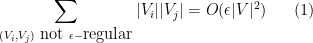
While Lemma 2 is, strictly speaking, weaker than Lemma 1 in that it does not enforce the equitable size property between the atoms, in practice it seems that the two lemmas are roughly of equal utility; most of the combinatorial consequences of Lemma 1 can also be proven using Lemma 2. The point is that one always has to remember to weight each cell by its density , rather than by giving each cell an equal weight as in Lemma 1. Lemma 2 also has the advantage that one can easily generalise the result from finite vertex sets to other probability spaces (for instance, one could weight with something other than the uniform distribution). For applications to hypergraph regularity, it turns out to be slightly more convenient to have two partitions (coarse and fine) rather than just one; see for instance my own paper on this topic. In any event the arguments below that we give to prove Lemma 2 can be modified to give a proof of Lemma 1 also. The proof of the regularity lemma is usually conducted by a greedy algorithm. Very roughly speaking, one starts with the trivial partition of . If this partition already regularises the graph, we are done; if not, this means that there are some sets and in which there is a significant density fluctuation beyond what has already been detected by the original partition. One then adds these sets to the partition and iterates the argument. Every time a new density fluctuation is incorporated into the partition that models the original graph, this increases a certain “index” or “energy” of the partition. On the other hand, this energy remains bounded no matter how complex the partition, so eventually one must reach a long “energy plateau” in which no further refinement is possible, at which point one can find the regular partition.

One disadvantage of the greedy algorithm is that it is not efficient in the limit , as it requires one to search over all pairs of subsets of a given pair of cells, which is an exponentially long search. There are more algorithmically efficient ways to regularise, for instance a polynomial time algorithm was given by Alon, Duke, Lefmann, Rödl, and Yuster. However, one can do even better, if one is willing to (a) allow cells of unequal size, (b) allow a small probability of failure, (c) have the ability to sample vertices from at random, and (d) allow for the cells to be defined “implicitly” (via their relationships with a fixed set of reference vertices) rather than “explicitly” (as a list of vertices). In that case, one can regularise a graph in a number of operations bounded in . Indeed, one has

Lemma 3 (Regularity lemma via random neighbourhoods) Let . Then there exists integers with the following property: whenever be a graph on finitely many vertices, if one selects one of the integers at random from , then selects vertices uniformly from at random, then the vertex cells (some of which can be empty) generated by the vertex neighbourhoods for , will obey the conclusions of Lemma 2 with probability at least .

Thus, roughly speaking, one can regularise a graph simply by taking a large number of random vertex neighbourhoods, and using the partition (or Venn diagram) generated by these neighbourhoods as the partition. The intuition is that if there is any non-uniformity in the graph (e.g. if the graph exhibits bipartite behaviour), this will bias the random neighbourhoods to seek out the partitions that would regularise that non-uniformity (e.g. vertex neighbourhoods would begin to fill out the two vertex cells associated to the bipartite property); if one takes sufficiently many such random neighbourhoods, the probability that all detectable non-uniformity is captured by the partition should converge to . (It is more complicated than this, because the finer one makes the partition, the finer the types of non-uniformity one can begin to detect, but this is the basic idea.)

This fact seems to be reasonably well-known folklore, discovered independently by many authors; it is for instance quite close to the graph property testing results of Alon and Shapira, and also appears implicitly in a paper of Ishigami, as well as a paper of Austin (and perhaps even more implicitly in a paper of myself). However, in none of these papers is the above lemma stated explicitly. I was asked about this lemma recently, so I decided to provide a proof here.