Ultraproducts as a Bridge Between Discrete and Continuous Analysis

(This is an extended blog post version of my talk “Ultraproducts as a Bridge Between Discrete and Continuous Analysis” that I gave at the Simons institute for the theory of computing at the workshop “Neo-Classical methods in discrete analysis“. Some of the material here is drawn from previous blog posts, notably “Ultraproducts as a bridge between hard analysis and soft analysis” and “Ultralimit analysis and quantitative algebraic geometry“‘. The text here has substantially more details than the talk; one may wish to skip all of the proofs given here to obtain a closer approximation to the original talk.)

Discrete analysis, of course, is primarily interested in the study of discrete (or “finitary”) mathematical objects: integers, rational numbers (which can be viewed as ratios of integers), finite sets, finite graphs, finite or discrete metric spaces, and so forth. However, many powerful tools in mathematics (e.g. ergodic theory, measure theory, topological group theory, algebraic geometry, spectral theory, etc.) work best when applied to continuous (or “infinitary”) mathematical objects: real or complex numbers, manifolds, algebraic varieties, continuous topological or metric spaces, etc. In order to apply results and ideas from continuous mathematics to discrete settings, there are basically two approaches. One is to directly discretise the arguments used in continuous mathematics, which often requires one to keep careful track of all the bounds on various quantities of interest, particularly with regard to various error terms arising from discretisation which would otherwise have been negligible in the continuous setting. The other is to construct continuous objects as limits of sequences of discrete objects of interest, so that results from continuous mathematics may be applied (often as a “black box”) to the continuous limit, which then can be used to deduce consequences for the original discrete objects which are quantitative (though often ineffectively so). The latter approach is the focus of this current talk.

The following table gives some examples of a discrete theory and its continuous counterpart, together with a limiting procedure that might be used to pass from the former to the latter:

(Discrete)	(Continuous)	(Limit method)
Ramsey theory	Topological dynamics	Compactness
Density Ramsey theory	Ergodic theory	Furstenberg correspondence principle
Graph/hypergraph regularity	Measure theory	Graph limits
Polynomial regularity	Linear algebra	Ultralimits
Structural decompositions	Hilbert space geometry	Ultralimits
Fourier analysis	Spectral theory	Direct and inverse limits
Quantitative algebraic geometry	Algebraic geometry	Schemes
Discrete metric spaces	Continuous metric spaces	Gromov-Hausdorff limits
Approximate group theory	Topological group theory	Model theory

As the above table illustrates, there are a variety of different ways to form a limiting continuous object. Roughly speaking, one can divide limits into three categories:

• Topological and metric limits. These notions of limits are commonly used by analysts. Here, one starts with a sequence (or perhaps a net) of objects in a common space , which one then endows with the structure of a topological space or a metric space, by defining a notion of distance between two points of the space, or a notion of open neighbourhoods or open sets in the space. Provided that the sequence or net is convergent, this produces a limit object , which remains in the same space, and is “close” to many of the original objects with respect to the given metric or topology.
• Categorical limits. These notions of limits are commonly used by algebraists. Here, one starts with a sequence (or more generally, a diagram) of objects in a category , which are connected to each other by various morphisms. If the ambient category is well-behaved, one can then form the direct limit or the inverse limit of these objects, which is another object in the same category , and is connected to the original objects by various morphisms.
• Logical limits. These notions of limits are commonly used by model theorists. Here, one starts with a sequence of objects or of spaces , each of which is (a component of) a model for given (first-order) mathematical language (e.g. if one is working in the language of groups, might be groups and might be elements of these groups). By using devices such as the ultraproduct construction, or the compactness theorem in logic, one can then create a new object or a new space , which is still a model of the same language (e.g. if the spaces were all groups, then the limiting space will also be a group), and is “close” to the original objects or spaces in the sense that any assertion (in the given language) that is true for the limiting object or space, will also be true for many of the original objects or spaces, and conversely. (For instance, if is an abelian group, then the will also be abelian groups for many .)

The purpose of this talk is to highlight the third type of limit, and specifically the ultraproduct construction, as being a “universal” limiting procedure that can be used to replace most of the limits previously mentioned. Unlike the topological or metric limits, one does not need the original objects to all lie in a common space in order to form an ultralimit ; they are permitted to lie in different spaces ; this is more natural in many discrete contexts, e.g. when considering graphs on vertices in the limit when goes to infinity. Also, no convergence properties on the are required in order for the ultralimit to exist. Similarly, ultraproduct limits differ from categorical limits in that no morphisms between the various spaces involved are required in order to construct the ultraproduct.

With so few requirements on the objects or spaces , the ultraproduct construction is necessarily a very “soft” one. Nevertheless, the construction has two very useful properties which make it particularly useful for the purpose of extracting good continuous limit objects out of a sequence of discrete objects. First of all, there is Łos’s theorem, which roughly speaking asserts that any first-order sentence which is asymptotically obeyed by the , will be exactly obeyed by the limit object ; in particular, one can often take a discrete sequence of “partial counterexamples” to some assertion, and produce a continuous “complete counterexample” that same assertion via an ultraproduct construction; taking the contrapositives, one can often then establish a rigorous equivalence between a quantitative discrete statement and its qualitative continuous counterpart. Secondly, there is the countable saturation property that ultraproducts automatically enjoy, which is a property closely analogous to that of compactness in topological spaces, and can often be used to ensure that the continuous objects produced by ultraproduct methods are “complete” or “compact” in various senses, which is particularly useful in being able to upgrade qualitative (or “pointwise”) bounds to quantitative (or “uniform”) bounds, more or less “for free”, thus reducing significantly the burden of “epsilon management” (although the price one pays for this is that one needs to pay attention to which mathematical objects of study are “standard” and which are “nonstandard”). To achieve this compactness or completeness, one sometimes has to restrict to the “bounded” portion of the ultraproduct, and it is often also convenient to quotient out the “infinitesimal” portion in order to complement these compactness properties with a matching “Hausdorff” property, thus creating familiar examples of continuous spaces, such as locally compact Hausdorff spaces.

Ultraproducts are not the only logical limit in the model theorist’s toolbox, but they are one of the simplest to set up and use, and already suffice for many of the applications of logical limits outside of model theory. In this post, I will set out the basic theory of these ultraproducts, and illustrate how they can be used to pass between discrete and continuous theories in each of the examples listed in the above table.

Apart from the initial “one-time cost” of setting up the ultraproduct machinery, the main loss one incurs when using ultraproduct methods is that it becomes very difficult to extract explicit quantitative bounds from results that are proven by transferring qualitative continuous results to the discrete setting via ultraproducts. However, in many cases (particularly those involving regularity-type lemmas) the bounds are already of tower-exponential type or worse, and there is arguably not much to be lost by abandoning the explicit quantitative bounds altogether.

Rectification and the Lefschetz principle

The rectification principle in arithmetic combinatorics asserts, roughly speaking, that very small subsets (or, alternatively, small structured subsets) of an additive group or a field of large characteristic can be modeled (for the purposes of arithmetic combinatorics) by subsets of a group or field of zero characteristic, such as the integers or the complex numbers . The additive form of this principle is known as the Freiman rectification principle; it has several formulations, going back of course to the original work of Freiman. Here is one formulation as given by Bilu, Lev, and Ruzsa:

Proposition 1 (Additive rectification) Let be a subset of the additive group for some prime , and let be an integer. Suppose that . Then there exists a map into a subset of the integers which is a Freiman isomorphism of order in the sense that for any , one has

if and only if

Furthermore is a right-inverse of the obvious projection homomorphism from to .

The original version of the rectification principle allowed the sets involved to be substantially larger in size (cardinality up to a small constant multiple of ), but with the additional hypothesis of bounded doubling involved; see the above-mentioned papers, as well as this later paper of Green and Ruzsa, for further discussion.

The proof of Proposition 1 is quite short (see Theorem 3.1 of Bilu-Lev-Ruzsa); the main idea is to use Minkowski’s theorem to find a non-trivial dilate of that is contained in a small neighbourhood of the origin in , at which point the rectification map can be constructed by hand.

Very recently, Codrut Grosu obtained an arithmetic analogue of the above theorem, in which the rectification map preserves both additive and multiplicative structure:

Theorem 2 (Arithmetic rectification) Let be a subset of the finite field for some prime , and let be an integer. Suppose that . Then there exists a map into a subset of the complex numbers which is a Freiman field isomorphism of order in the sense that for any and any polynomial of degree at most and integer coefficients of magnitude summing to at most , one has

if and only if

Note that it is necessary to use an algebraically closed field such as for this theorem, in contrast to the integers used in Proposition 1, as can contain objects such as square roots of which can only map to in the complex numbers (once is at least ).

Using Theorem 2, one can transfer results in arithmetic combinatorics (e.g. sum-product or Szemerédi-Trotter type theorems) regarding finite subsets of to analogous results regarding sufficiently small subsets of ; see the paper of Grosu for several examples of this. This should be compared with the paper of Vu, Wood, and Wood, which introduces a converse principle that embeds finite subsets of (or more generally, a characteristic zero integral domain) in a Freiman field-isomorphic fashion into finite subsets of for arbitrarily large primes , allowing one to transfer arithmetic combinatorical facts from the latter setting to the former.

Grosu’s argument uses some quantitative elimination theory, and in particular a quantitative variant of a lemma of Chang that was discussed previously on this blog. In that previous blog post, it was observed that (an ineffective version of) Chang’s theorem could be obtained using only qualitative algebraic geometry (as opposed to quantitative algebraic geometry tools such as elimination theory results with explicit bounds) by means of nonstandard analysis (or, in what amounts to essentially the same thing in this context, the use of ultraproducts). One can then ask whether one can similarly establish an ineffective version of Grosu’s result by nonstandard means. The purpose of this post is to record that this can indeed be done without much difficulty, though the result obtained, being ineffective, is somewhat weaker than that in Theorem 2. More precisely, we obtain

Theorem 3 (Ineffective arithmetic rectification) Let . Then if is a field of characteristic at least for some depending on , and is a subset of of cardinality , then there exists a map into a subset of the complex numbers which is a Freiman field isomorphism of order .

Our arguments will not provide any effective bound on the quantity (though one could in principle eventually extract such a bound by deconstructing the proof of Proposition 4 below), making this result weaker than Theorem 2 (save for the minor generalisation that it can handle fields of prime power order as well as fields of prime order as long as the characteristic remains large).

Following the principle that ultraproducts can be used as a bridge to connect quantitative and qualitative results (as discussed in these previous blog posts), we will deduce Theorem 3 from the following (well-known) qualitative version:

Proposition 4 (Baby Lefschetz principle) Let be a field of characteristic zero that is finitely generated over the rationals. Then there is an isomorphism from to a subfield of .

This principle (first laid out in an appendix of Lefschetz’s book), among other things, often allows one to use the methods of complex analysis (e.g. Riemann surface theory) to study many other fields of characteristic zero. There are many variants and extensions of this principle; see for instance this MathOverflow post for some discussion of these. I used this baby version of the Lefschetz principle recently in a paper on expanding polynomial maps.

Proof: We give two proofs of this fact, one using transcendence bases and the other using Hilbert’s nullstellensatz.

We begin with the former proof. As is finitely generated over , it has finite transcendence degree, thus one can find algebraically independent elements of over such that is a finite extension of , and in particular by the primitive element theorem is generated by and an element which is algebraic over . (Here we use the fact that characteristic zero fields are separable.) If we then define by first mapping to generic (and thus algebraically independent) complex numbers , and then setting to be a complex root of of the minimal polynomial for over after replacing each with the complex number , we obtain a field isomorphism with the required properties.

Now we give the latter proof. Let be elements of that generate that field over , but which are not necessarily algebraically independent. Our task is then equivalent to that of finding complex numbers with the property that, for any polynomial with rational coefficients, one has

if and only if

Let be the collection of all polynomials with rational coefficients with , and be the collection of all polynomials with rational coefficients with . The set

is the intersection of countably many algebraic sets and is thus also an algebraic set (by the Hilbert basis theorem or the Noetherian property of algebraic sets). If the desired claim failed, then could be covered by the algebraic sets for . By decomposing into irreducible varieties and observing (e.g. from the Baire category theorem) that a variety of a given dimension over cannot be covered by countably many varieties of smaller dimension, we conclude that must in fact be covered by a finite number of such sets, thus

for some . By the nullstellensatz, we thus have an identity of the form

for some natural numbers , polynomials , and polynomials with coefficients in . In particular, this identity also holds in the algebraic closure of . Evaluating this identity at we see that the right-hand side is zero but the left-hand side is non-zero, a contradiction, and the claim follows.

From Proposition 4 one can now deduce Theorem 3 by a routine ultraproduct argument (the same one used in these previous blog posts). Suppose for contradiction that Theorem 3 fails. Then there exists natural numbers , a sequence of finite fields of characteristic at least , and subsets of of cardinality such that for each , there does not exist a Freiman field isomorphism of order from to the complex numbers. Now we select a non-principal ultrafilter , and construct the ultraproduct of the finite fields . This is again a field (and is a basic example of what is known as a pseudo-finite field); because the characteristic of goes to infinity as , it is easy to see (using Los’s theorem) that has characteristic zero and can thus be viewed as an extension of the rationals .

Now let be the ultralimit of the , so that is the ultraproduct of the , then is a subset of of cardinality . In particular, if is the field generated by and , then is a finitely generated extension of the rationals and thus, by Proposition 4 there is an isomorphism from to a subfield of the complex numbers. In particular, are complex numbers, and for any polynomial with integer coefficients, one has

if and only if

By Los’s theorem, we then conclude that for all sufficiently close to , one has for all polynomials of degree at most and whose coefficients are integers whose magnitude sums up to , one has

if and only if

But this gives a Freiman field isomorphism of order between and , contradicting the construction of , and Theorem 3 follows.

Multiple recurrence in quasirandom groups

I’ve just uploaded to the arXiv my joint paper with Vitaly Bergelson, “Multiple recurrence in quasirandom groups“, which is submitted to Geom. Func. Anal.. This paper builds upon a paper of Gowers in which he introduced the concept of a quasirandom group, and established some mixing (or recurrence) properties of such groups. A -quasirandom group is a finite group with no non-trivial unitary representations of dimension at most . We will informally refer to a “quasirandom group” as a -quasirandom group with the quasirandomness parameter large (more formally, one can work with a sequence of -quasirandom groups with going to infinity). A typical example of a quasirandom group is where is a large prime. Quasirandom groups are discussed in depth in this blog post. One of the key properties of quasirandom groups established in Gowers’ paper is the following “weak mixing” property: if are subsets of , then for “almost all” , one has

where denotes the density of in . Here, we use to informally represent an estimate of the form (where is a quantity that goes to zero when the quasirandomness parameter goes to infinity), and “almost all ” denotes “for all in a subset of of density “. As a corollary, if have positive density in (by which we mean that is bounded away from zero, uniformly in the quasirandomness parameter , and similarly for ), then (if the quasirandomness parameter is sufficiently large) we can find elements such that , , . In fact we can find approximately such pairs . To put it another way: if we choose uniformly and independently at random from , then the events , , are approximately independent (thus the random variable resembles a uniformly distributed random variable on in some weak sense). One can also express this mixing property in integral form as

for any bounded functions . (Of course, with being finite, one could replace the integrals here by finite averages if desired.) Or in probabilistic language, we have

where are drawn uniformly and independently at random from .

As observed in Gowers’ paper, one can iterate this observation to find “parallelopipeds” of any given dimension in dense subsets of . For instance, applying (1) with replaced by , , and one can assert (after some relabeling) that for chosen uniformly and independently at random from , the events , , , , , , are approximately independent whenever are dense subsets of ; thus the tuple resebles a uniformly distributed random variable in in some weak sense.

However, there are other tuples for which the above iteration argument does not seem to apply. One of the simplest tuples in this vein is the tuple in , when are drawn uniformly at random from a quasirandom group . Here, one does not expect the tuple to behave as if it were uniformly distributed in , because there is an obvious constraint connecting the last two components of this tuple: they must lie in the same conjugacy class! In particular, if is a subset of that is the union of conjugacy classes, then the events , are perfectly correlated, so that is equal to rather than . Our main result, though, is that in a quasirandom group, this is (approximately) the only constraint on the tuple. More precisely, we have

Theorem 1 Let be a -quasirandom group, and let be drawn uniformly at random from . Then for any , we have

where goes to zero as , are drawn uniformly and independently at random from , and is drawn uniformly at random from the conjugates of for each fixed choice of .

This is the probabilistic formulation of the above theorem; one can also phrase the theorem in other formulations (such as an integral formulation), and this is detailed in the paper. This theorem leads to a number of recurrence results; for instance, as a corollary of this result, we have

for almost all , and any dense subsets of ; the lower and upper bounds are sharp, with the lower bound being attained when is randomly distributed, and the upper bound when is conjugation-invariant.

To me, the more interesting thing here is not the result itself, but how it is proven. Vitaly and I were not able to find a purely finitary way to establish this mixing theorem. Instead, we had to first use the machinery of ultraproducts (as discussed in this previous post) to convert the finitary statement about a quasirandom group to an infinitary statement about a type of infinite group which we call an ultra quasirandom group (basically, an ultraproduct of increasingly quasirandom finite groups). This is analogous to how the Furstenberg correspondence principle is used to convert a finitary combinatorial problem into an infinitary ergodic theory problem.

Ultra quasirandom groups come equipped with a finite, countably additive measure known as Loeb measure , which is very analogous to the Haar measure of a compact group, except that in the case of ultra quasirandom groups one does not quite have a topological structure that would give compactness. Instead, one has a slightly weaker structure known as a -topology, which is like a topology except that open sets are only closed under countable unions rather than arbitrary ones. There are some interesting measure-theoretic and topological issues regarding the distinction between topologies and -topologies (and between Haar measure and Loeb measure), but for this post it is perhaps best to gloss over these issues and pretend that ultra quasirandom groups come with a Haar measure. One can then recast Theorem 1 as a mixing theorem for the left and right actions of the ultra approximate group on itself, which roughly speaking is the assertion that

for “almost all” , if are bounded measurable functions on , with having zero mean on all conjugacy classes of , where are the left and right translation operators

To establish this mixing theorem, we use the machinery of idempotent ultrafilters, which is a particularly useful tool for understanding the ergodic theory of actions of countable groups that need not be amenable; in the non-amenable setting the classical ergodic averages do not make much sense, but ultrafilter-based averages are still available. To oversimplify substantially, the idempotent ultrafilter arguments let one establish mixing estimates of the form (2) for “many” elements of an infinite-dimensional parallelopiped known as an IP system (provided that the actions of this IP system obey some technical mixing hypotheses, but let’s ignore that for sake of this discussion). The claim then follows by using the quasirandomness hypothesis to show that if the estimate (2) failed for a large set of , then this large set would then contain an IP system, contradicting the previous claim.

Idempotent ultrafilters are an extremely infinitary type of mathematical object (one has to use Zorn’s lemma no fewer than three times just to construct one of these objects!). So it is quite remarkable that they can be used to establish a finitary theorem such as Theorem 1, though as is often the case with such infinitary arguments, one gets absolutely no quantitative control whatsoever on the error terms appearing in that theorem. (It is also mildly amusing to note that our arguments involve the use of ultrafilters in two completely different ways: firstly in order to set up the ultraproduct that converts the finitary mixing problem to an infinitary one, and secondly to solve the infinitary mixing problem. Despite some superficial similarities, there appear to be no substantial commonalities between these two usages of ultrafilters.) There is already a fair amount of literature on using idempotent ultrafilter methods in infinitary ergodic theory, and perhaps by further development of ultraproduct correspondence principles, one can use such methods to obtain further finitary consequences (although the state of the art for idempotent ultrafilter ergodic theory has not advanced much beyond the analysis of two commuting shifts currently, which is the main reason why our arguments only handle the pattern and not more sophisticated patterns).

We also have some miscellaneous other results in the paper. It turns out that by using the triangle removal lemma from graph theory, one can obtain a recurrence result that asserts that whenever is a dense subset of a finite group (not necessarily quasirandom), then there are pairs such that all lie in . Using a hypergraph generalisation of the triangle removal lemma known as the hypergraph removal lemma, one can obtain more complicated versions of this statement; for instance, if is a dense subset of , then one can find triples such that all lie in . But the method is tailored to the specific types of patterns given here, and we do not have a general method for obtaining recurrence or mixing properties for arbitrary patterns of words in some finite alphabet such as .

We also give some properties of a model example of an ultra quasirandom group, namely the ultraproduct of where is a sequence of primes going off to infinity. Thanks to the substantial recent progress (by Helfgott, Bourgain, Gamburd, Breuillard, and others) on understanding the expansion properties of the finite groups , we have a fair amount of knowledge on the ultraproduct as well; for instance any two elements of will almost surely generate a spectral gap. We don’t have any direct application of this particular ultra quasirandom group, but it might be interesting to study it further.

Definable subsets over (nonstandard) finite fields, and almost quantifier elimination

Much as group theory is the study of groups, or graph theory is the study of graphs, model theory is the study of models (also known as structures) of some language (which, in this post, will always be a single-sorted, first-order language). A structure is a set , equipped with one or more operations, constants, and relations. This is of course an extremely general type of mathematical object, but (quite remarkably) one can still say a substantial number of interesting things about very broad classes of structures.

We will observe the common abuse of notation of using the set as a metonym for the entire structure, much as we usually refer to a group simply as , a vector space simply as , and so forth. Following another common bending of the rules, we also allow some operations on structures (such as the multiplicative inverse operation on a group or field) to only be partially defined, and we allow use of the usual simplifying conventions for mathematical formulas (e.g. writing instead of or , in cases where associativity is known). We will also deviate slightly from the usual practice in logic by emphasising individual structures, rather than the theory of general classes of structures; for instance, we will talk about the theory of a single field such as or , rather than the theory of all fields of a certain type (e.g. real closed fields or algebraically closed fields).

Once one has a structure , one can introduce the notion of a definable subset of , or more generally of a Cartesian power of , defined as a set of the form

for some formula in the language with free variables and any number of constants from (that is, is a well-formed formula built up from a finite number of constants in , the relations and operations on , logical connectives such as , , , and the quantifiers ). Thus, for instance, in the theory of the arithmetic of the natural numbers , the set of primes is a definable set, since we have

In the theory of the field of reals , the unit circle is an example of a definable set,

but so is the the complement of the circle,

and the interval :

Due to the unlimited use of constants, any finite subset of a power of any structure is, by our conventions, definable in that structure. (One can of course also consider definability without parameters (also known as -definability), in which arbitrary constants are not permitted, but we will not do so here.)

We can isolate some special subclasses of definable sets:

• An atomic definable set is a set of the form (1) in which is an atomic formula (i.e. it does not contain any logical connectives or quantifiers).
• A quantifier-free definable set is a set of the form (1) in which is quantifier-free (i.e. it can contain logical connectives, but does not contain the quantifiers ).

Example 1 In the theory of a field such as , an atomic definable set is the same thing as an affine algebraic set (also known as an affine algebraic variety, with the understanding that varieties are not necessarily assumed to be irreducible), and a quantifier-free definable set is known as a constructible set; thus we see that algebraic geometry can be viewed in some sense as a special case of model theory. (Conversely, it can in fact be quite profitable to think of model theory as an abstraction of algebraic geometry; for instance, the concepts of Morley rank and Morley degree in model theory (discussed in this previous blog post) directly generalises the concepts of dimension and degree in algebraic geometry.) Over , the interval is a definable set, but not a quantifier-free definable set (and certainly not an atomic definable set); and similarly for the primes over .

A quantifier-free definable set in is nothing more than a finite boolean combination of atomic definable sets; in other words, the class of quantifier-free definable sets over is the smallest class that contains the atomic definable sets and is closed under boolean operations such as complementation and union (which generate all the other boolean operations). Similarly, the class of definable sets over is the smallest class that contains the quantifier-free definable sets, and is also closed under the operation of projection from to for every natural number , where is the map .

Some structures have the property of enjoying quantifier elimination, which means that every definable set is in fact a quantifier-free definable set, or equivalently that the projection of a quantifier-free definable set is again quantifier-free. For instance, an algebraically closed field (with the field operations) has quantifier elimination (i.e. the projection of a constructible set is again constructible); this fact can be proven by the classical tool of resultants, and among other things can be used to give a proof of Hilbert’s nullstellensatz. (Note though that projection does not necessary preserve the property of being atomic; for instance, the projection of the atomic set is the non-atomic, but still quantifier-free definable, set .) In the converse direction, it is not difficult to use the nullstellensatz to deduce quantifier elimination. For theory of the real field , which is not algebraically closed, one does not have quantifier elimination, as one can see from the example of the unit circle (which is a quantifier-free definable set) projecting down to the interval (which is definable, but not quantifer-free definable). However, if one adds the additional operation of order to the reals, giving it the language of an ordered field rather than just a field, then quantifier elimination is recovered (the class of quantifier-free definable sets now enlarges to match the class of definable sets, which in this case is also the class of semi-algebraic sets); this is the famous Tarski-Seidenberg theorem.

On the other hand, many important structures do not have quantifier elimination; typically, the projection of a quantifier-free definable set is not, in general, quantifier-free definable. This failure of the projection property also shows up in many contexts outside of model theory; for instance, Lebesgue famously made the error of thinking that the projection of a Borel measurable set remained Borel measurable (it is merely an analytic set instead). Turing’s halting theorem can be viewed as an assertion that the projection of a decidable set (also known as a computable or recursive set) is not necessarily decidable (it is merely semi-decidable (or recursively enumerable) instead). The notorious P=NP problem can also be essentially viewed in this spirit; roughly speaking (and glossing over the placement of some quantifiers), it asks whether the projection of a polynomial-time decidable set is again polynomial-time decidable. And so forth. (See this blog post of Dick Lipton for further discussion of the subtleties of projections.)

Now we consider the status of quantifier elimination for the theory of a finite field . If interpreted naively, quantifier elimination is trivial for a finite field , since every subset of is finite and thus quantifier-free definable. However, we can recover an interesting question in one of two (essentially equivalent) ways. One is to work in the asymptotic regime in which the field is large, but the length of the formulae used to construct one’s definable sets stays bounded uniformly in the size of (where we view any constant in as contributing a unit amount to the length of a formula, no matter how large is). A simple counting argument then shows that only a small number of subsets of become definable in the asymptotic limit , since the number of definable sets clearly grows at most polynomially in for any fixed bound on the formula length, while the number of all subsets of grows exponentially in .

Another way to proceed is to work not with a single finite field , or even with a sequence of finite fields, but with the ultraproduct of a sequence of finite fields, and to study the properties of definable sets over this ultraproduct. (We will be using the notation of ultraproducts and nonstandard analysis from this previous blog post.) This approach is equivalent to the more finitary approach mentioned in the previous paragraph, at least if one does not care to track of the exact bounds on the length of the formulae involved. Indeed, thanks to Los’s theorem, a definable subset of is nothing more than the ultraproduct of definable subsets of for all sufficiently close to , with the length of the formulae used to define uniformly bounded in . In the language of nonstandard analysis, one can view as a nonstandard finite field.

The ultraproduct of finite fields is an important example of a pseudo-finite field – a field that obeys all the sentences in the languages of fields that finite fields do, but is not necessarily itself a finite field. The model theory of pseudo-finite fields was first studied systematically by Ax (in the same paper where the Ax-Grothendieck theorem, discussed previously on this blog, was established), with important further contributions by Kiefe, by Fried-Sacerdote, by two papers of Chatzidakis-van den Dries-Macintyre, and many other authors.

As mentioned before, quantifier elimination trivially holds for finite fields. But for infinite pseudo-finite fields, such as the ultraproduct of finite fields with going to infinity, quantifier elimination fails. For instance, in a finite field , the set of quadratic residues is a definable set, with a bounded formula length, and so in the ultraproduct , the set of nonstandard quadratic residues is also a definable set. However, in one dimension, we see from the factor theorem that the only atomic definable sets are either finite or the whole field , and so the only constructible sets (i.e. the only quantifier-free definable sets) are either finite or cofinite in . Since the quadratic residues have asymptotic density in a large finite field, they cannot form a quantifier-free definable set, despite being definable.

Nevertheless, there is a very nice almost quantifier elimination result for these fields, in characteristic zero at least, which we phrase here as follows:

Theorem 1 (Almost quantifier elimination) Let be a nonstandard finite field of characteristic zero, and let be a definable set over . Then is the union of finitely many sets of the form

where is an atomic definable subset of (i.e. the -points of an algebraic variety defined over in ) and is a polynomial.

Results of this type were first obtained essentially due to Catarina Kiefe, although the formulation here is closer to that of Chatzidakis-van den Dries-Macintyre.

Informally, this theorem says that while we cannot quite eliminate all quantifiers from a definable set over a nonstandard finite field, we can eliminate all but one existential quantifier. Note that negation has also been eliminated in this theorem; for instance, the definable set uses a negation, but can also be described using a single existential quantifier as .) I believe that there are more complicated analogues of this result in positive characteristic, but I have not studied this case in detail (Kiefe’s result does not assume characteristic zero, but her conclusion is slightly different from the one given here). In the one-dimensional case , the only varieties are the affine line and finite sets, and we can simplify the above statement, namely that any definable subset of takes the form for some polynomial (i.e. definable sets in are nothing more than the projections of the -points of a plane curve).

There is an equivalent formulation of this theorem for standard finite fields, namely that if is a finite field and is definable using a formula of length at most , then can be expressed in the form (2) with the degree of bounded by some quantity depending on and , assuming that the characteristic of is sufficiently large depending on .

The theorem gives quite a satisfactory description of definable sets in either standard or nonstandard finite fields (at least if one does not care about effective bounds in some of the constants, and if one is willing to exclude the small characteristic case); for instance, in conjunction with the Lang-Weil bound discussed in this recent blog post, it shows that any non-empty definable subset of a nonstandard finite field has a nonstandard cardinality of for some positive standard rational and integer . Equivalently, any non-empty definable subset of for some standard finite field using a formula of length at most has a standard cardinality of for some positive rational of height and some natural number between and . (For instance, in the example of the quadratic residues given above, is equal to and equal to .) There is a more precise statement to this effect, namely that the Poincaré series of a definable set is rational; see Kiefe’s paper for details.

Below the fold I give a proof of Theorem 1, which relies primarily on the Lang-Weil bound mentioned above.

254B, Notes 5: Product theorems, pivot arguments, and the Larsen-Pink non-concentration inequality

In the previous set of notes, we saw that one could derive expansion of Cayley graphs from three ingredients: non-concentration, product theorems, and quasirandomness. Quasirandomness was discussed in Notes 3. In the current set of notes, we discuss product theorems. Roughly speaking, these theorems assert that in certain circumstances, a finite subset of a group either exhibits expansion (in the sense that , say, is significantly larger than ), or is somehow “close to” or “trapped” by a genuine group.

Theorem 1 (Product theorem in ) Let , let be a finite field, and let be a finite subset of . Let be sufficiently small depending on . Then at least one of the following statements holds:

• (Expansion) One has .
• (Close to ) One has .
• (Trapping) is contained in a proper subgroup of .

We will prove this theorem (which was proven first in the cases for fields of prime order by Helfgott, and then for and general by Dinai, and finally to general and independently by Pyber-Szabo and by Breuillard-Green-Tao) later in this notes. A more qualitative version of this proposition was also previously obtained by Hrushovski. There are also generalisations of the product theorem of importance to number theory, in which the field is replaced by a cyclic ring (with not necessarily prime); this was achieved first for and square-free by Bourgain, Gamburd, and Sarnak, by Varju for general and square-free, and finally by this paper of Bourgain and Varju for arbitrary and .

Exercise 1 (Diameter bound) Assuming Theorem 1, show that whenever is a symmetric set of generators of for some finite field and some , then any element of can be expressed as the product of elements from . (Equivalently, if we add the identity element to , then for some .) This is a special case of a conjecture of Babai and Seress, who conjectured that the bound should hold uniformly for all finite simple groups (in particular, the implied constants here should not actually depend on . The methods used to handle the case can handle other finite groups of Lie type of bounded rank, but at present we do not have bounds that are independent of the rank. On the other hand, a recent paper of Helfgott and Seress has almost resolved the conjecture for the permutation groups .

A key tool to establish product theorems is an argument which is sometimes referred to as the pivot argument. To illustrate this argument, let us first discuss a much simpler (and older) theorem, essentially due to Freiman, which has a much weaker conclusion but is valid in any group :

Theorem 2 (Baby product theorem) Let be a group, and let be a finite non-empty subset of . Then one of the following statements hold:

• (Expansion) One has .
• (Close to a subgroup) is contained in a left-coset of a group with .

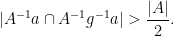
To prove this theorem, we suppose that the first conclusion does not hold, thus . Our task is then to place inside the left-coset of a fairly small group .

To do this, we take a group element , and consider the intersection . A priori, the size of this set could range from anywhere from to . However, we can use the hypothesis to obtain an important dichotomy, reminiscent of the classical fact that two cosets of a subgroup of are either identical or disjoint:

Proposition 3 (Dichotomy) If , then exactly one of the following occurs:

• (Non-involved case) is empty.
• (Involved case) .

Proof: Suppose we are not in the pivot case, so that is non-empty. Let be an element of , then and both lie in . The sets and then both lie in . As these sets have cardinality and lie in , which has cardinality less than , we conclude from the inclusion-exclusion formula that

But the left-hand side is equal to , and the claim follows.

The above proposition provides a clear separation between two types of elements : the “non-involved” elements, which have nothing to do with (in the sense that , and the “involved” elements, which have a lot to do with (in the sense that . The key point is that there is a significant “gap” between the non-involved and involved elements; there are no elements that are only “slightly involved”, in that and intersect a little but not a lot. It is this gap that will allow us to upgrade approximate structure to exact structure. Namely,

Proposition 4 The set of involved elements is a finite group, and is equal to .

Proof: It is clear that the identity element is involved, and that if is involved then so is (since . Now suppose that are both involved. Then and have cardinality greater than and are both subsets of , and so have non-empty intersection. In particular, is non-empty, and so is non-empty. By Proposition 3, this makes involved. It is then clear that is a group.

If , then is non-empty, and so from Proposition 3 is involved. Conversely, if is involved, then . Thus we have as claimed. In particular, is finite.

Now we can quickly wrap up the proof of Theorem 2. By construction, for all ,which by double counting shows that . As , we see that is contained in a right coset of ; setting , we conclude that is contained in a left coset of . is a conjugate of , and so . If , then and both lie in and have cardinality , so must overlap; and so . Thus , and so , and Theorem 2 follows.

Exercise 2 Show that the constant in Theorem 2 cannot be replaced by any larger constant.

Exercise 3 Let be a finite non-empty set such that . Show that . (Hint: If , show that for some .)

Exercise 4 Let be a finite non-empty set such that . Show that there is a finite group with and a group element such that and .

Below the fold, we give further examples of the pivot argument in other group-like situations, including Theorem 2 and also the “sum-product theorem” of Bourgain-Katz-Tao and Bourgain-Glibichuk-Konyagin.

254A, Notes 6: Ultraproducts as a bridge between hard analysis and soft analysis

Roughly speaking, mathematical analysis can be divided into two major styles, namely hard analysis and soft analysis. The precise distinction between the two types of analysis is imprecise (and in some cases one may use a blend the two styles), but some key differences can be listed as follows.

• Hard analysis tends to be concerned with quantitative or effective properties such as estimates, upper and lower bounds, convergence rates, and growth rates or decay rates. In contrast, soft analysis tends to be concerned with qualitative or ineffective properties such as existence and uniqueness, finiteness, measurability, continuity, differentiability, connectedness, or compactness.
• Hard analysis tends to be focused on finitary, finite-dimensional or discrete objects, such as finite sets, finitely generated groups, finite Boolean combination of boxes or balls, or “finite-complexity” functions, such as polynomials or functions on a finite set. In contrast, soft analysis tends to be focused on infinitary, infinite-dimensional, or continuous objects, such as arbitrary measurable sets or measurable functions, or abstract locally compact groups.
• Hard analysis tends to involve explicit use of many parameters such as , , , etc. In contrast, soft analysis tends to rely instead on properties such as continuity, differentiability, compactness, etc., which implicitly are defined using a similar set of parameters, but whose parameters often do not make an explicit appearance in arguments.
• In hard analysis, it is often the case that a key lemma in the literature is not quite optimised for the application at hand, and one has to reprove a slight variant of that lemma (using a variant of the proof of the original lemma) in order for it to be suitable for applications. In contrast, in soft analysis, key results can often be used as “black boxes”, without need of further modification or inspection of the proof.
• The properties in soft analysis tend to enjoy precise closure properties; for instance, the composition or linear combination of continuous functions is again continuous, and similarly for measurability, differentiability, etc. In contrast, the closure properties in hard analysis tend to be fuzzier, in that the parameters in the conclusion are often different from the parameters in the hypotheses. For instance, the composition of two Lipschitz functions with Lipschitz constant is still Lipschitz, but now with Lipschitz constant instead of . These changes in parameters mean that hard analysis arguments often require more “bookkeeping” than their soft analysis counterparts, and are less able to utilise algebraic constructions (e.g. quotient space constructions) that rely heavily on precise closure properties.

In the lectures so far, focusing on the theory surrounding Hilbert’s fifth problem, the results and techniques have fallen well inside the category of soft analysis. However, we will now turn to the theory of approximate groups, which is a topic which is traditionally studied using the methods of hard analysis. (Later we will also study groups of polynomial growth, which lies on an intermediate position in the spectrum between hard and soft analysis, and which can be profitably analysed using both styles of analysis.)

Despite the superficial differences between hard and soft analysis, though, there are a number of important correspondences between results in hard analysis and results in soft analysis. For instance, if one has some sort of uniform quantitative bound on some expression relating to finitary objects, one can often use limiting arguments to then conclude a qualitative bound on analogous expressions on infinitary objects, by viewing the latter objects as some sort of “limit” of the former objects. Conversely, if one has a qualitative bound on infinitary objects, one can often use compactness and contradiction arguments to recover uniform quantitative bounds on finitary objects as a corollary.

Remark 1 Another type of correspondence between hard analysis and soft analysis, which is “syntactical” rather than “semantical” in nature, arises by taking the proofs of a soft analysis result, and translating such a qualitative proof somehow (e.g. by carefully manipulating quantifiers) into a quantitative proof of an analogous hard analysis result. This type of technique is sometimes referred to as proof mining in the proof theory literature, and is discussed in this previous blog post (and its comments). We will however not employ systematic proof mining techniques here, although in later posts we will informally borrow arguments from infinitary settings (such as the methods used to construct Gleason metrics) and adapt them to finitary ones.

Let us illustrate the correspondence between hard and soft analysis results with a simple example.

Proposition 1 Let be a sequentially compact topological space, let be a dense subset of , and let be a continuous function (giving the extended half-line the usual order topology). Then the following statements are equivalent:

• (i) (Qualitative bound on infinitary objects) For all , one has .
• (ii) (Quantitative bound on finitary objects) There exists such that for all .

In applications, is typically a (non-compact) set of “finitary” (or “finite complexity”) objects of a certain class, and is some sort of “completion” or “compactification” of which admits additional “infinitary” objects that may be viewed as limits of finitary objects.

Proof: To see that (ii) implies (i), observe from density that every point in is adherent to , and so given any neighbourhood of , there exists . Since , we conclude from the continuity of that also, and the claim follows.

Conversely, to show that (i) implies (ii), we use the “compactness and contradiction” argument. Suppose for sake of contradiction that (ii) failed. Then for any natural number , there exists such that . (Here we have used the axiom of choice, which we will assume throughout this course.) Using sequential compactness, and passing to a subsequence if necessary, we may assume that the converge to a limit . By continuity of , this implies that , contradicting (i).

Remark 2 Note that the above deduction of (ii) from (i) is ineffective in that it gives no explicit bound on the uniform bound in (ii). Without any further information on how the qualitative bound (i) is proven, this is the best one can do in general (and this is one of the most significant weaknesses of infinitary methods when used to solve finitary problems); but if one has access to the proof of (i), one can often finitise or proof mine that argument to extract an effective bound for , although often the bound one obtains in the process is quite poor (particularly if the proof of (i) relied extensively on infinitary tools, such as limits). See this blog post for some related discussion.

The above simple example illustrates that in order to get from an “infinitary” statement such as (i) to a “finitary” statement such as (ii), a key step is to be able to take a sequence (or in some cases, a more general net ) of finitary objects and extract a suitable infinitary limit object . In the literature, there are three main ways in which one can extract such a limit:

• (Topological limit) If the are all elements of some topological space (e.g. an incomplete function space) which has a suitable “compactification” or “completion” (e.g. a Banach space), then (after passing to a subsequence if necessary) one can often ensure the converge in a topological sense (or in a metrical sense) to a limit . The use of this type of limit to pass between quantitative/finitary and qualitative/infinitary results is particularly common in the more analytical areas of mathematics (such as ergodic theory, asymptotic combinatorics, or PDE), due to the abundance of useful compactness results in analysis such as the (sequential) Banach-Alaoglu theorem, Prokhorov’s theorem, the Helly selection theorem, the Arzelá-Ascoli theorem, or even the humble Bolzano-Weierstrass theorem. However, one often has to take care with the nature of convergence, as many compactness theorems only guarantee convergence in a weak sense rather than in a strong one.
• (Categorical limit) If the are all objects in some category (e.g. metric spaces, groups, fields, etc.) with a number of morphisms between the (e.g. morphisms from to , or vice versa), then one can often form a direct limit or inverse limit of these objects to form a limiting object . The use of these types of limits to connect quantitative and qualitative results is common in subjects such as algebraic geometry that are particularly amenable to categorical ways of thinking. (We have seen inverse limits appear in the discussion of Hilbert’s fifth problem, although in that context they were not really used to connect quantitative and qualitative results together.)
• (Logical limit) If the are all distinct spaces (or elements or subsets of distinct spaces), with few morphisms connecting them together, then topological and categorical limits are often unavailable or unhelpful. In such cases, however, one can still tie together such objects using an ultraproduct construction (or similar device) to create a limiting object or limiting space that is a logical limit of the , in the sense that various properties of the (particularly those that can be phrased using the language of first-order logic) are preserved in the limit. As such, logical limits are often very well suited for the task of connecting finitary and infinitary mathematics together. Ultralimit type constructions are of course used extensively in logic (particularly in model theory), but are also popular in metric geometry. They can also be used in many of the previously mentioned areas of mathematics, such as algebraic geometry (as discussed in this previous post).

The three types of limits are analogous in many ways, with a number of connections between them. For instance, in the study of groups of polynomial growth, both topological limits (using the metric notion of Gromov-Hausdorff convergence) and logical limits (using the ultralimit construction) are commonly used, and to some extent the two constructions are at least partially interchangeable in this setting. (See also these previous posts for the use of ultralimits as a substitute for topological limits.) In the theory of approximate groups, though, it was observed by Hrushovski that logical limits (and in particular, ultraproducts) are the most useful type of limit to connect finitary approximate groups to their infinitary counterparts. One reason for this is that one is often interested in obtaining results on approximate groups that are uniform in the choice of ambient group . As such, one often seeks to take a limit of approximate groups that lie in completely unrelated ambient groups , with no obvious morphisms or metrics tying the to each other. As such, the topological and categorical limits are not easily usable, whereas the logical limits can still be employed without much difficulty.

Logical limits are closely tied with non-standard analysis. Indeed, by applying an ultraproduct construction to standard number systems such as the natural numbers or the reals , one can obtain nonstandard number systems such as the nonstandard natural numbers or the nonstandard real numbers (or hyperreals) . These nonstandard number systems behave very similarly to their standard counterparts, but also enjoy the advantage of containing the standard number systems as proper subsystems (e.g. is a subring of ), which allows for some convenient algebraic manipulations (such as the quotient space construction to create spaces such as ) which are not easily accessible in the purely standard universe. Nonstandard spaces also enjoy a useful completeness property, known as countable saturation, which is analogous to metric completeness (as discussed in this previous blog post) and which will be particularly useful for us in tying together the theory of approximate groups with the theory of Hilbert’s fifth problem. See this previous post for more discussion on ultrafilters and nonstandard analysis.

In these notes, we lay out the basic theory of ultraproducts and ultralimits (in particular, proving Los’s theorem, which roughly speaking asserts that ultralimits are limits in a logical sense, as well as the countable saturation property alluded to earlier). We also lay out some of the basic foundations of nonstandard analysis, although we will not rely too heavily on nonstandard tools in this course. Finally, we apply this general theory to approximate groups, to connect finite approximate groups to an infinitary type of approximate group which we will call an ultra approximate group. We will then study these ultra approximate groups (and models of such groups) in more detail in the next set of notes.

Remark 3 Throughout these notes (and in the rest of the course), we will assume the axiom of choice, in order to easily use ultrafilter-based tools. If one really wanted to expend the effort, though, one could eliminate the axiom of choice from the proofs of the final “finitary” results that one is ultimately interested in proving, at the cost of making the proofs significantly lengthier. Indeed, there is a general result of Gödel that any result which can be stated in the language of Peano arithmetic (which, roughly speaking, means that the result is “finitary” in nature), and can be proven in set theory using the axiom of choice (or more precisely, in the ZFC axiom system), can also be proven in set theory without the axiom of choice (i.e. in the ZF system). As this course is not focused on foundations, we shall simply assume the axiom of choice henceforth to avoid further distraction by such issues.