The Lang-Weil bound

Let be a finite field, with algebraic closure , and let be an (affine) algebraic variety defined over , by which I mean a set of the form

for some ambient dimension , and some finite number of polynomials . In order to reduce the number of subscripts later on, let us say that has complexity at most if , , and the degrees of the are all less than or equal to . Note that we do not require at this stage that be irreducible (i.e. not the union of two strictly smaller varieties), or defined over , though we will often specialise to these cases later in this post. (Also, everything said here can also be applied with almost no changes to projective varieties, but we will stick with affine varieties for sake of concreteness.)

One can consider two crude measures of how “big” the variety is. The first measure, which is algebraic geometric in nature, is the dimension of the variety , which is an integer between and (or, depending on convention, , , or undefined, if is empty) that can be defined in a large number of ways (e.g. it is the largest for which the generic linear projection from to is dominant, or the smallest for which the intersection with a generic codimension subspace is non-empty). The second measure, which is number-theoretic in nature, is the number of -points of , i.e. points in all of whose coefficients lie in the finite field, or equivalently the number of solutions to the system of equations for with variables in .

These two measures are linked together in a number of ways. For instance, we have the basic Schwarz-Zippel type bound (which, in this qualitative form, goes back at least to Lemma 1 of the work of Lang and Weil in 1954).

Lemma 1 (Schwarz-Zippel type bound) Let be a variety of complexity at most . Then we have .

Proof: (Sketch) For the purposes of exposition, we will not carefully track the dependencies of implied constants on the complexity , instead simply assuming that all of these quantities remain controlled throughout the argument. (If one wished, one could obtain ineffective bounds on these quantities by an ultralimit argument, as discussed in this previous post, or equivalently by moving everything over to a nonstandard analysis framework; one could also obtain such uniformity using the machinery of schemes.)

We argue by induction on the ambient dimension of the variety . The case is trivial, so suppose and that the claim has already been proven for . By breaking up into irreducible components we may assume that is irreducible (this requires some control on the number and complexity of these components, but this is available, as discussed in this previous post). For each , the fibre is either one-dimensional (and thus all of ) or zero-dimensional. In the latter case, one has points in the fibre from the fundamental theorem of algebra (indeed one has a bound of in this case), and lives in the projection of to , which is a variety of dimension at most and controlled complexity, so the contribution of this case is acceptable from the induction hypothesis. In the former case, the fibre contributes -points, but lies in a variety in of dimension at most (since otherwise would contain a subvariety of dimension at least , which is absurd) and controlled complexity, and so the contribution of this case is also acceptable from the induction hypothesis.

One can improve the bound on the implied constant to be linear in the degree of (see e.g. Claim 7.2 of this paper of Dvir, Kollar, and Lovett, or Lemma A.3 of this paper of Ellenberg, Oberlin, and myself), but we will not be concerned with these improvements here.

Without further hypotheses on , the above upper bound is sharp (except for improvements in the implied constants). For instance, the variety

where are distict, is the union of distinct hyperplanes of dimension , with and complexity ; similar examples can easily be concocted for other choices of . In the other direction, there is also no non-trivial lower bound for without further hypotheses on . For a trivial example, if is an element of that does not lie in , then the hyperplane

clearly has no -points whatsoever, despite being a -dimensional variety in of complexity . For a slightly less non-trivial example, if is an element of that is not a quadratic residue, then the variety

which is the union of two hyperplanes, still has no -points, even though this time the variety is defined over instead of (by which we mean that the defining polynomial(s) have all of their coefficients in ). There is however the important Lang-Weil bound that allows for a much better estimate as long as is both defined over and irreducible:

Theorem 2 (Lang-Weil bound) Let be a variety of complexity at most . Assume that is defined over , and that is irreducible as a variety over (i.e. is geometrically irreducible or absolutely irreducible). Then

Again, more explicit bounds on the implied constant here are known, but will not be the focus of this post. As the previous examples show, the hypotheses of definability over and geometric irreducibility are both necessary.

The Lang-Weil bound is already non-trivial in the model case of plane curves:

Theorem 3 (Hasse-Weil bound) Let be an irreducible polynomial of degree with coefficients in . Then

Thus, for instance, if , then the elliptic curve has -points, a result first established by Hasse. The Hasse-Weil bound is already quite non-trivial, being the analogue of the Riemann hypothesis for plane curves. For hyper-elliptic curves, an elementary proof (due to Stepanov) is discussed in this previous post. For general plane curves, the first proof was by Weil (leading to his famous Weil conjectures); there is also a nice version of Stepanov’s argument due to Bombieri covering this case which is a little less elementary (relying crucially on the Riemann-Roch theorem for the upper bound, and a lifting trick to then get the lower bound), which I briefly summarise later in this post. The full Lang-Weil bound is deduced from the Hasse-Weil bound by an induction argument using generic hyperplane slicing, as I will also summarise later in this post.

The hypotheses of definability over and geometric irreducibility in the Lang-Weil can be removed after inserting a geometric factor:

Corollary 4 (Lang-Weil bound, alternate form) Let be a variety of complexity at most . Then one has

where is the number of top-dimensional components of (i.e. geometrically irreducible components of of dimension ) that are definable over , or equivalently are invariant with respect to the Frobenius endomorphism that defines .

Proof: By breaking up a general variety into components (and using Lemma 1 to dispose of any lower-dimensional components), it suffices to establish this claim when is itself geometrically irreducible. If is definable over , the claim follows from Theorem 2. If is not definable over , then it is not fixed by the Frobenius endomorphism (since otherwise one could produce a set of defining polynomials that were fixed by Frobenius and thus defined over by using some canonical basis (such as a reduced Grobner basis) for the associated ideal), and so has strictly smaller dimension than . But captures all the -points of , so in this case the claim follows from Lemma 1.

Note that if is reducible but is itself defined over , then the Frobenius endomorphism preserves itself, but may permute the components of around. In this case, is the number of fixed points of this permutation action of Frobenius on the components. In particular, is always a natural number between and ; thus we see that regardless of the geometry of , the normalised count is asymptotically restricted to a bounded range of natural numbers (in the regime where the complexity stays bounded and goes to infinity).

Example 1 Consider the variety

for some non-zero parameter . Geometrically (by which we basically mean “when viewed over the algebraically closed field “), this is the union of two lines, with slopes corresponding to the two square roots of . If is a quadratic residue, then both of these lines are defined over , and are fixed by Frobenius, and in this case. If is not a quadratic residue, then the lines are not defined over , and the Frobenius automorphism permutes the two lines while preserving as a whole, giving in this case.

Corollary 4 effectively computes (at least to leading order) the number-theoretic size of a variety in terms of geometric information about , namely its dimension and the number of top-dimensional components fixed by Frobenius. It turns out that with a little bit more effort, one can extend this connection to cover not just a single variety , but a family of varieties indexed by points in some base space . More precisely, suppose we now have two affine varieties of bounded complexity, together with a regular map of bounded complexity (the definition of complexity of a regular map is a bit technical, see e.g. this paper, but one can think for instance of a polynomial or rational map of bounded degree as a good example). It will be convenient to assume that the base space is irreducible. If the map is a dominant map (i.e. the image is Zariski dense in ), then standard algebraic geometry results tell us that the fibres are an unramified family of -dimensional varieties outside of an exceptional subset of of dimension strictly smaller than (and with having dimension strictly smaller than ); see e.g. Section I.6.3 of Shafarevich.

Now suppose that , , and are defined over . Then, by Lang-Weil, has -points, and by Schwarz-Zippel, for all but of these -points (the ones that lie in the subvariety ), the fibre is an algebraic variety defined over of dimension . By using ultraproduct arguments (see e.g. Lemma 3.7 of this paper of mine with Emmanuel Breuillard and Ben Green), this variety can be shown to have bounded complexity, and thus by Corollary 4, has -points. One can then ask how the quantity is distributed. A simple but illustrative example occurs when and is the polynomial . Then equals when is a non-zero quadratic residue and when is a non-zero quadratic non-residue (and when is zero, but this is a negligible fraction of all ). In particular, in the asymptotic limit , is equal to half of the time and half of the time.

Now we describe the asymptotic distribution of the . We need some additional notation. Let be an -point in , and let be the connected components of the fibre . As is defined over , this set of components is permuted by the Frobenius endomorphism . But there is also an action by monodromy of the fundamental group (this requires a certain amount of étale machinery to properly set up, as we are working over a positive characteristic field rather than over the complex numbers, but I am going to ignore this rather important detail here, as I still don’t fully understand it). This fundamental group may be infinite, but (by the étale construction) is always profinite, and in particular has a Haar probability measure, in which every finite index subgroup (and their cosets) are measurable. Thus we may meaningfully talk about elements drawn uniformly at random from this group, so long as we work only with the profinite -algebra on that is generated by the cosets of the finite index subgroups of this group (which will be the only relevant sets we need to measure when considering the action of this group on finite sets, such as the components of a generic fibre).

Theorem 5 (Lang-Weil with parameters) Let be varieties of complexity at most with irreducible, and let be a dominant map of complexity at most . Let be an -point of . Then, for any natural number , one has for values of , where is the random variable that counts the number of components of a generic fibre that are invariant under , where is an element chosen uniformly at random from the étale fundamental group . In particular, in the asymptotic limit , and with chosen uniformly at random from , (or, equivalently, ) and have the same asymptotic distribution.

This theorem generalises Corollary 4 (which is the case when is just a point, so that is just and is trivial). Informally, the effect of a non-trivial parameter space on the Lang-Weil bound is to push around the Frobenius map by monodromy for the purposes of counting invariant components, and a randomly chosen set of parameters corresponds to a randomly chosen loop on which to perform monodromy.

Example 2 Let and for some fixed ; to avoid some technical issues let us suppose that is coprime to . Then can be taken to be , and for a base point we can take . The fibre – the roots of unity – can be identified with the cyclic group by using a primitive root of unity. The étale fundamental group is (I think) isomorphic to the profinite closure of the integers (excluding the part of that closure coming from the characteristic of ). Not coincidentally, the integers are the fundamental group of the complex analogue of . (Brian Conrad points out to me though that for more complicated varieties, such as covers of by a power of the characteristic, the etale fundamental group is more complicated than just a profinite closure of the ordinary fundamental group, due to the presence of Artin-Schreier covers that are only ramified at infinity.) The action of this fundamental group on the fibres can given by translation. Meanwhile, the Frobenius map on is given by multiplication by . A random element then becomes a random affine map on , where chosen uniformly at random from . The number of fixed points of this map is equal to the greatest common divisor of and when is divisible by , and equal to otherwise. This matches up with the elementary number fact that a randomly chosen non-zero element of will be an power with probability , and when this occurs, the number of roots in will be .

Example 3 (Thanks to Jordan Ellenberg for this example.) Consider a random elliptic curve , where are chosen uniformly at random, and let . Let be the -torsion points of (i.e. those elements with using the elliptic curve addition law); as a group, this is isomorphic to (assuming that has sufficiently large characteristic, for simplicity), and consider the number of points of , which is a random variable taking values in the natural numbers between and . In this case, the base variety is the modular curve , and the covering variety is the modular curve . The generic fibre here can be identified with , the monodromy action projects down to the action of , and the action of Frobenius on this fibre can be shown to be given by a matrix with determinant (with the exact choice of matrix depending on the choice of fibre and of the identification), so the distribution of the number of -points of is asymptotic to the distribution of the number of fixed points of a random linear map of determinant on .

Theorem 5 seems to be well known “folklore” among arithmetic geometers, though I do not know of an explicit reference for it. I enjoyed deriving it for myself (though my derivation is somewhat incomplete due to my lack of understanding of étale cohomology) from the ordinary Lang-Weil theorem and the moment method. I’m recording this derivation later in this post, mostly for my own benefit (as I am still in the process of learning this material), though perhaps some other readers may also be interested in it.

Caveat: not all details are fully fleshed out in this writeup, particularly those involving the finer points of algebraic geometry and étale cohomology, as my understanding of these topics is not as complete as I would like it to be.

Many thanks to Brian Conrad and Jordan Ellenberg for helpful discussions on these topics.

— 1. The Stepanov-Bombieri proof of the Hasse-Weil bound —

We now give (most of) the Stepanov-Bombieri proof of Theorem 3, following the exposition of Bombieri (see also these lecture notes of Kowalski, focusing on the model case of curves of the form ). In this section all implied constants are allowed to depend on the degree of the polynomial .

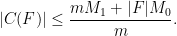
Let be the -points of the curve ; the hypothesis that is irreducible means that the curve is also irreducible. Our task is to establish the upper bound

and the lower bound

For technical reasons, we only prove these bounds directly when is a perfect square; the general case then follows by using the explicit formula for as a function of and the tensor power trick, as explained in this previous post.

Now we prove the upper bound. One uses Stepanov’s polynomial method (discussed in these previous blog posts, for a somewhat different set of applications). The basic idea here is to bound the size of a finite set by constructing a non-trivial polynomial of controlled degree that vanishes to high order at each point of . Stepanov’s original argument projected the curve onto an affine line so that one could use ordinary one-dimensional polynomials, but Bombieri’s approach works directly on the curve . For this it becomes convenient to work in the language of divisors of rational functions, rather than zeroes of polynomials (and also it becomes slightly more convenient to work projectively rather than affinely, though I will gloss over this minor detail). Given a rational function on the curve (with coefficients in ) that is not identically zero or identically infinite on , one can define the divisor to be the formal sum of the zeroes and poles of on , weighted by the multiplicity of the zero or pole (with poles being viewed as having negative multiplicity; one has to be a little careful defining multiplicity at singular points of , but this can be done by using a sufficiently algebraic formalism). The irreducibility of (which, of course, must be used at some juncture to prove the Hasse-Weil bound) ensures that this formal sum only has finitely many non-zero terms. One can show that the total signed multiplicities of zeroes and poles of always add up to zero: . (This generalises the fundamental theorem of algebra, which is the case when is a projective line.)

Fix a point of (which one can think of as being at infinity), and for each degree , let be the space of those rational functions which are either zero, or have , i.e. has a pole of order at but no other poles; this generalises the space of polynomials of degree at most , which corresponds to the case when is a projective line and is the point at infinity. It is easy to see that is a vector space (over ), which is non-decreasing in . In the case when is a line, this space clearly has dimension . The Riemann-Roch theorem is the generalisation of this to the case of a general curve. In its most precise form, it asserts the identity

where is the genus of , and is the canonical divisor of (i.e. the divisor of the canonical line bundle of ). For our application, we will need two specific corollaries of the Riemann-Roch theorem, coming from the non-negativity and monotonicity properties of . The first is the Riemann inequality

(so in particular ), and the second is the inequality

for all . In particular, if we set to be the set of all degrees such that , then consists of all but at most elements of the natural numbers, and we can find a sequence of rational functions on with (i.e. has a pole of order exactly at and no other poles), with each being spanned by the with . The can be viewed as a generalisation of the standard monomial basis of the polynomials of one variable. A key point here is that the degrees of this basis are all distinct; this will be crucial later on for ensuring that the polynomial we will be using for Stepanov’s method does not vanish identically.

We will not prove the Riemann-Roch theorem here, and simply assume it (and its consequences) as a black box. Next, we consider the Frobenius map defined by . As is defined over , this map preserves , and the fixed points of this map are precisely the -points of .

The plan is now to find a non-trivial element for some controlled that vanishes to order at least at each fixed point of on for some . As the total number of zeroes and poles of must agree, this forces

and by optimising the parameters this should lead to (1).

The trick is to pick rational functions of a specific form, namely

where is a parameter to be optimised later, and for each , lies in for another parameter to be optimised in later. We also pick to divide , thus is a power of the characteristic of that is less than or equal to . There are several reasons to working with polynomials of this form. The first is that because of the Frobenius endomorphism identity , and divides by hypothesis, each term in is an power, and hence (since in characteristic ) is itself the power of some rational function. As such, whenever vanishes at a point, it automatically vanishes to order at least .

Secondly, in order for to vanish at every fixed point of the Frobenius map on (and thus vanish to order at each such point, by the above discussion), it is of course necessary and sufficient that the rational function

This is a constraint on the which is linear over (because the map is linear over , though not over ), and so we can try to enforce this constraint by linear algebra. Note that if each lies in , then the rational function on the left-hand side of of (4) lies in , so the vanishing (4) imposes homogeneous linear constraints (possibly dependent) over on the , where . On the other hand, the dimension (over ) of the space of all possible is

Thus, by linear algebra, we can find a collection of , not all zero, obeying (4) as long as we have

We are not done yet, because even if the are are not all zero, it is conceivable that the combined function (3) could still vanish. But observe that if is the largest index for which is non-zero, then the rational function has a pole of order at least at , and all the other terms have a pole of order at most (here it is crucial that the have poles of different orders at , thanks to Riemann-Roch). So as long as we have

we have that does not vanish identically. As it vanishes to degree at least at every point of , and lies in , and so we obtain the upper bound

Now we optimise in the parameters subject to the constraints (5), (6). As is assumed to be a perfect square and is sufficiently large, then a little work shows that one can satisfy the constraints with , , and for some sufficiently large , leading to the desired bound (1).

Remark 1 When is not a perfect square, but is not a prime, one can still choose other values of and obtain a weaker version of (1) that is still non-trivial. But it is curious that Bombieri’s version of Stepanov’s argument breaks down completely when has prime order. As mentioned previously, one can still recover this case a posteriori by the tensor product trick, but this requires the explicit formula for which is not exactly trivial. On the other hand, other versions of Stepanov’s argument (such as the one given in this previous blog post) do work in the prime order case, so this obstruction may be purely artificial in nature.

Now we need to pass from the upper bound (1) to the lower bound (2). In model cases, such as curves of the form with not divisible by the characteristic of , one can proceed by observing that the multiplicative group foliates into cosets of the subgroup of powers. Because of this, we see that the union of the curves contains exactly -points on all but vertical lines , , and hence the union has cardinality -points. (In other words, the projection from to is generically -to-one. Also, as the are all dilations of , they will be irreducible if is, and thus by (1) they each have at most -points; from subtracting all but one of the curves from we then see that each of the has at least -points also. As we can take one of the to be the identity, the claim (2) follows in this case. The general case follows in a similar fashion, using Galois theory to lifting a general curve to another curve whose projection to some coordinate line has fixed multiplicity (basically by ensuring that the function field of the former is a Galois extension of the function field of the latter); see Bombieri’s paper for details.

— 2. The proof of the Lang-Weil bound —

Now we prove the Lang-Weil bound. We allow all implied constants to depend on the complexity bound , and will ignore the issues of how to control the complexity of the various algebraic objects that arise in our analysis (as before, one can obtain such bounds more or less “for free” from an ultraproduct argument, if desired).

The proof proceeds by induction on the dimension of the variety . The first non-trivial case occurs at dimension one. If is a plane curve (so , and the ambient dimension is ), then the claim follows directly from the Hasse-Weil bound. If is a higher-dimensional curve, we can use resultants to eliminate all but two of the variables (or, alternatively, one can apply the primitive element theorem to the function field of the curve), and convert the curve to a birationally equivalent (over ) plane curve, to reduce to the plane curve case (noting that the singular points of the birational transformation only influence the number of -points by at most).

Now suppose inductively that , and that the claim has already been proven for irreducible varieties of dimension . The induction step is then based on the following two parallel facts about hyperplane slicing, the first in the algebraic geometric category, and the second in the combinatorial category:

Lemma 6 (Bertini’s theorem) Let be an irreducible variety in of dimension at least two. Then, for a generic affine hyperplane (over ), the slice is an irreducible variety of dimension .

Lemma 7 (Random sampling) Let be a subset of for some . Then, for a affine hyperplane (defined over ) chosen uniformly at random, the random variable has mean and variance . In particular, by Chebyshev’s inequality, the median value of is .

Let us see how the two lemmas conclude the induction. There are different affine hyperplanes over . The set of hyperplanes over for which fails to be an irreducible variety of dimension is, by Bertini’s theorem, a proper algebraic variety in the Grassmannian space, which one can show to have bounded complexity; and so by Lemma 1, only of all such hyperplanes over fall into this variety. For the remaining such hyperplanes, we may apply the induction hypothesis and conclude that . In particular, if is an affine hyperplane chosen uniformly at random, then the median value of is . But this is consistent with Lemma 7 only when , closing the induction.

Remark 2 One can also proceed without the variance bound in Lemma 7 by using Lemma 1 as a crude estimate for for the exceptional , after first making an easy reduction to the case where is not already contained inside a single hyperplane. However, I think the variance bound is illuminating, as it illustrates the concentration of measure that occurs when becomes much larger than , which only occurs in dimensions two and higher. In contrast, if one attempts to slice a curve by a hyperplane, one typically gets zero or multiple points, so there is no concentration of measure and irreducibility usually fails. So the slicing method can reduce the dimension of down to one, but not to zero, so the need to invoke Hasse-Weil cannot be avoided by this method.

We first show Lemma 7, which is a routine first and second moment calculation. Any given point in lies in precisely of the hyperplanes , so summing in we obtain . Next, any two distinct points in lie in of the hyperplanes , and so

giving the variance bound.

Now we show Bertini’s theorem. A dimension count shows that the space of pairs where is a hyperplane and is a singular point of in has dimension at most , and so for a generic hyperplane, the space of singular points of in is contained in a variety of dimension at most . Similarly, the space of pairs where is a smooth point of and is a hyperplane containing the tangent space to at is at most , and so the space of smooth points of in whose tangent space is not transverse to a generic also has dimension at most . Thus, for generic , the slice is a -dimensional variety, which is generically comes from smooth points of whose tangent space is transverse to . The remaining task is to establish irreducibility for generic . As irreducibility is an algebraic condition, is either generically irreducible or generically reducible. Suppose for contradiction that is generically reducible. Consider the set of triples where are distinct smooth points of , and is a hyperplane through that is transverse to the tangent spaces of both and , with reducible. This is a quasiprojective variety of dimension . It can be decomposed into two top-dimensional components: one where lie in the same component of , and one where they lie in distinct components. (The hypothesis is crucial to ensure that the first component is non-empty.) As such, is disconnected in the Zariski topology. On the other hand, for fixed , the set of all contributing to is connected, while the set of all distinct smooth pairs is also connected, and so (and hence is closure) is also connected, a contradiction.

Remark 3 See also page 174 of Griffiths-Harris for a slight variant of this argument (thanks to Jordan Ellenberg for pointing this out). In that reference, it is also noted that the claim can also be derived from the Lefschetz hyperplane theorem in the case that is smooth.

— 3. Lang-Weil with parameters —

Now we prove Theorem 5. Again we allow all implied constants to depend on the complexity parameter , and gloss over the task of making sure that all algebraic objects have complexity .

We will proceed by the moment method. Observe that is a bounded natural number random variable, so to show that has the asymptotic distribution of up to errors of , it suffices to show that

for any fixed natural number , or equivalently (by the Lang-Weil bound for and for the fibres )

Fix . We form the -fold fibre product of over , consisting of all -tuples such that lies in . This fibre product is a quasiprojective variety of dimension , is defined over , and the left-hand side of (7) is precisely equal to the number of -points of . Thus, by the Lang-Weil bound for , it suffices to show that

i.e. that has precisely top-dimensional components which are Frobenius-invariant.

We will in fact prove a more general statement: if is any dominant map which has smooth unramified fibres on , then the number of top-dimensional components of that are Frobenius-invariant is equal to the expected number of top-dimensional components of on a generic fibre , where is selected uniformly at random from . Specialising this to the fibre product (noting that the generic fibre of is just the -fold Cartesian power of the generic fibre of , and similarly for the action of Frobenius and the fundamental group), we obtain the claim.

Now we prove this more general statement. By decomposing into irreducible components, we may certainly assume that is irreducible. If is not Frobenius-invariant, then is generically disjoint from and so there certainly can be no components of that are fixed by . Thus we may assume that is Frobenius-invariant (i.e. defined over ). Then the situation becomes very close to that of Burnside’s lemma. If there are components of , the connectedness of implies that the fundamental group acts transitively on these components, and so for any single component and uniformly chosen , will be uniformly distributed amongst the , as will . In particular, each has a chance of being a fixed point of , so the expected number of fixed points of is as requred.

Exercise 1 Obtain the following extension of Corollary 5: if one has different dominant maps of varieties of complexity , with unramified, non-singular fibres on , then the joint distribution of converges in distribution to the joint distribution of , where each is the number of fixed points of on the components of a generic fibre, where is independent of and drawn uniformly from .

Remark 4 While the moment computation is simple and cute, I would be interested in seeing either a heuristic or rigorous explanation of Theorem 5 (or Exercise 1) that did not proceed through moments. The theorem seems to be asserting a statement roughly of the following form (ignoring for now the fact that paths do not actually make much sense in positive characteristic): if one takes a random path in connecting two random -points, then the loop behaves as if it is distributed uniformly in the fundamental group of (or , for any lower-dimensional set ). But I do not know how to make this heuristic precise.