
For much of last week I was in Leiden, Holland, giving one of the Ostrowski prize lectures at the annual meeting of the Netherlands mathematical congress. My talk was not on the subject of the prize (arithmetic progressions in primes), as this was covered by a talk of Ben Green there, but rather on a certain “uniform uncertainty principle” in Fourier analysis, and its relation to compressed sensing; this is work which is joint with Emmanuel Candes and also partly with Justin Romberg.
As mentioned in the previous post here, compressed sensing is a relatively new measurement paradigm which seeks to capture the “essential” aspects of a high-dimensional object using as few measurements as possible. There are many contexts in which compressed sensing is potentially useful, but for this talk (which is focussed on theory rather than applications) I will just consider a single toy model arising from Fourier analysis. Specifically, the object we seek to measure will be a complex function 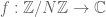


We suppose that we can measure some (but perhaps not all) of the Fourier coefficients of f, and ask whether we can reconstruct f from this information; the objective is to use as few Fourier coefficients as possible. More specifically, we fix a set 
- Let N be a known integer, let
be an unknown function, let
be a sequence of known Fourier coefficients of f for all
. Is it possible to reconstruct f uniquely from this information?
- If so, what is a practical algorithm for finding f?
For instance, if 


which can be computed quite quickly, for instance by using the fast Fourier transform.
Now we ask what happens when 


However, we can hope to recover unique solvability for this problem by making an additional hypothesis on the function f. There are many such hypotheses one could make, but for this toy problem we shall simply assume that f is sparse. Specifically, we fix an integer S between 1 and N, and say that a function f is S-sparse if f is non-zero in at most S places, or equivalently if the support 
- Let S and N be known integers, let
be an unknown S-sparse function, let
- If so, what is a practical algorithm for finding f?
Note that while we know how sparse f is, we are not given to know exactly where f is sparse – there are S positions out of the N total positions where f might be non-zero, but we do not know which S positions these are. The fact that the support is not known a priori is one of the key difficulties with this problem. Nevertheless, setting that problem aside for the moment, we see that f now has only S degrees of freedom instead of N, and so by repeating the previous analysis one might now hope that the answer to Q1 becomes yes as soon as 
Actually, one needs at least 


One might hope that this necessary condition is close to being sharp, so that the answer to the modified Q1 is yes as soon as
Uncertainty principle (informal): If a function is sparse and not identically zero, then its Fourier transform should be non-sparse.
This type of principle is motivated by the Heisenberg uncertainty principle in physics; the size of the support of f is a proxy for the spatial uncertainty of f, whereas the size of the support of 
Discrete uncertainty principle: If f is not identically zero, then
.
Proof: Combine the Plancherel identity
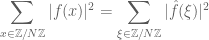
with the elementary inequalities

and


By applying this principle we see that we obtain unique recoverability as soon as 
There are cases in which the condition 


One can concoct several further counterexamples of this type, but they require various subgroups of
Chebotarev lemma: Let N be prime. Then every square minor of the Fourier matrix
is invertible.
This lemma has been rediscovered or reproved at least seven times in the literature (I myself rediscovered it once); there is a nice survey paper on Chebotarev’s work which summarises some of this. (A nice connection to the setting of this talk, pointed out to me by Hendrik Lenstra here at Leiden: Chebotarev’s lemma was originally conjectured to be true by Ostrowski.) As a quick corollary of this lemma, we obtain the following improvement to the uncertainty principle in the prime order case.
Uncertainty principle for cyclic groups of prime order: If N is prime and f is not identically zero, then
.
From this one can quickly show that one does indeed obtain unique recoverability for S-sparse functions in cyclic groups of prime order whenever one has
This settles the (modified) Q1 posed above, at least for groups of prime order. But it does not settle Q2 – the question of exactly how one recovers f from the given data 
- Brute force. If we knew precisely what the support
of f was, we can use linear algebra methods to solve for f in terms of the coefficients
, since we have
of these) and apply linear algebra to each combination. This works, but is horribly computationally expensive, and is completely impractical once N and S are of any reasonable size, e.g. larger than 1000.
minimisation. Out of all the possible functions f which match the given data (i.e.
for all
. This works too, but is still impractical: the general problem of finding the sparsest solution to a linear system of equations contains the infamous subset sum decision problem as a special case (we’ll leave this as an exercise to the reader) and so this problem is NP-hard in general. (Note that this does not imply that the original problem Q1 is similarly NP-hard, because that problem involves a specific linear system, which turns out to be rather different from the specific linear system used to encode subset-sum.)
minimisation (i.e. the method of least squares). Out of all the possible functions f which match the given data, find the one of least energy, i.e. which minimises the
. This method has the advantage (unlike 1 and 2) of being extremely easy to carry out; indeed, the minimiser is given explicitly by the formula
. Unfortunately, this minimiser not guaranteed at all to be S-sparse, and indeed the uncertainty principle suggests in fact that the
So we have two approaches to Q2 which work but are computationally infeasible, and one approach which is computationally feasible but doesn’t work. It turns out however that one can take a “best of both worlds” approach halfway between method 2 and method 3, namely:
minimisation (or basis pursuit): Out of all the possible functions f which match the given data, find the one of least energy, i.e. which minimises the
.
The key difference between this minimisation problem and the
Before we reveal the answer, we can at least give an informal geometric argument as to why
It turns out that if 

The above counterexamples used very structured examples of sets of observed frequencies 
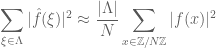
Uniform Uncertainty Principle (UUP): If Lambda is a random set with
, then with overwhelming probability (at least
for any fixed A), we have the approximate local Plancherel identity
for all 4S-sparse functions f, where by
we mean that X and Y differ by at most 10%. (N is not required to be prime.)
The above formulation is a little imprecise; see this paper (which had 

By using this principle (and variants of this principle), one can indeed show that basis pursuit works:
Theorem [CRT], [CT]. Suppose
. Then any given S-sparse function f will be recovered exactly by
Roughly speaking, the idea in the latter result is to use the UUP to show that the Fourier coefficients of any sparse (or
The method is rather robust; there is some followup work which demonstrates stability of the basis pursuit method with respect to several types of noise. See also the ICM proceedings article of Emmanuel Candes for a recent survey. It can also be abstracted from this toy Fourier problem to a more general problem of recovering sparse or compressible data from few measurements. As long as the measurement matrix obeys an appropriate generalisation of the UUP, the basis pursuit methods are quite effective (both in theory, in numerical experiments, and more recently in laboratory prototypes).

43 comments
Comments feed for this article
16 April, 2007 at 8:00 am
Igor Carron
Thank you for this post. I am not a mathematician so please forgive my ignorance on that subject matter but you said:
“..For a single function f, this type of localisation of the Plancherel identity… uses the same phenomena that explain why Monte Carlo integration is so effective.”
Do you mean to say that Monte Carlo integration is working well because the function to be integrated is sparse ? In the affirmative, does this mean that if I were to know better the sparsity of a function to be integrated using a Monte Carlo technique, I could, in principle, accelerate the convergence rate of that integration ?
16 April, 2007 at 10:03 am
Terence Tao
Dear Igor,
Here we are summing the Fourier transform of f (or more precisely, ) rather than f itself. The uncertainty principle tells us that as f is sparse, the Fourier transform of f should be “smooth” or “structured” (or “low complexity”). For these types of functions, Monte Carlo integration works rather well (though there are other integration schemes that are even faster).
Compressed sensing methods are only moderately fast from a computational perspective; their main strength lies in the fact that they can give accurate results (after reasonable amounts of computation) from relatively small amounts of data; they are thus valuable in situations where computation is relatively cheap but measurement is expensive. These types of algorithms, for instance, would allow one to compute the integral of a function f exactly (not just approximately) if one knew that the Fourier transform of f was sparse, and one sampled f at a fairly small number of randomly chosen values. (In fact, one would recover all of f, not just its integral.)
16 April, 2007 at 11:18 am
Igor Carron
Thank you for your time.
20 April, 2007 at 8:03 pm
Weiyu Xu
It is very nice to see you remain active in the compressive sensing area.
This topic is very interesting, but I would like to know what open problems still look interesting to the applied mathematics and singal processing society? It seems to me that most have been done,… I would appreciate it if you can share with us your opinions about the future directions of the compressive sensing area.
21 April, 2007 at 8:22 am
Terence Tao
Dear Weiyu,
It appears to me that research in this area is now being primarily driven by fairly concrete applications (imaging, MRI, etc.) rather than by theory; in particular, there is a lot of work on efficient implementation of algorithms, numerical simulation, testing on real-world signals, etc. But there are still some interesting theoretical questions of a rather vague and broad nature – these types of applied fields don’t seem to lend themselves to the kind of precise conjectures one sees in pure mathematics. One is derandomisation; all of the measurement ensembles for which the really strong compressed sensing results are known have to be generated by a random process; no deterministic compressed sensing method which is rigorously backed by theory is known. Another question is to see whether one can improve the two basic algorithms of basis pursuit and matching pursuit and obtain better results (in either accuracy, speed, or robustness); given the lack of lower bounds in this subject it is difficult to tell how close the current algorithms are to being optimal. A third is to relax the hypotheses on the measurement ensemble, in particular to allow for some limited amount of linear dependence (or near-dependence) between columns of the measuremement matrix.
22 April, 2007 at 10:26 am
Sri Hari
Dear Tao,
I am novice in the field of mathematics and I want to ask what do you mean by “degrees of freedom” of a function space ? Is it the number of complex exponentials which make the signal I mean is it the dimension of the Fourier basis?
Thank you
23 April, 2007 at 7:38 am
Terence Tao
In this case, yes. More generally, degrees of freedom refer to the number of independent real numbers one needs to fully describe the state of an object; it can be made precise with various mathematical notions of “dimension” but in this post I am using it mostly in an informal heuristic sense.
24 April, 2007 at 8:24 am
oz
Thanx a lot for two very interesting posts.
I have a problem which appears to be conceptually similar to the ‘compressed sensing’ problems.
The problem is finding a sparse convex representation:
Suppose you’re given m points a_1,.., a_m in R^n with m > > n.
You’re also given a point b which is a sparse convex combination of the points, i.e. b = \sum_{i} x_i a_i where the x_i’s are non-negative and sum to one, and only k of them are non-zero (k < n, but still too large to enumerate all sets of k points …). The goal is to find the weights x –
this amounts to finding a sparse positive solution for Ax=b, (here A is the matrix whose columns are a_1,..,a_m) so to me it looks like the setting mentioned in the post, and my guess is that the two approaches (i.e. ‘greedy’ and ‘convex optimization’) could work here.
Any suggestions/known results for this problem?
Thanx,
oz
24 April, 2007 at 11:07 am
Terence Tao
Dear Oz,
Assuming that the a_1,…,a_m are dispersed more or less randomly, it seems that one can simply plug in either of the two algorithms mentioned above to find a sparse solution to Ax=b. It is not a priori positive, but if k < < n and the a_1,…,a_m are in general position then there can be at most one k-sparse solution, so if a k-sparse positive solution exists, this method will find it (assuming that the hypotheses necessary for the reconstruction method to work are satisfied, of course).
One could add the positivity constraints to the linear program one solves for the basis pursuit method, but my guess is that this will not significantly improve performance, though one should try some numerical experiments both ways to see if this is the case.
30 April, 2007 at 6:03 am
Utpal Sarkar
Dear Terence,
Do you know if your uncertainty principle for cyclic groups of prime order generalizes to general finite abelian groups if you restrict to functions whose support is not contained in any proper subgroup?
Thanks,
Utpal
30 April, 2007 at 7:53 am
Terence Tao
Dear Uptal,
That’s an interesting question; I don’t have any counterexample to your conjecture (though one should probably look first at ). As I said in the main post, the best uncertainty principle for arbitrary groups known is by Meshulam, and it is not well understood exactly how sharp his estimates are (though I believe they are quite sharp for p-groups). Such a result also seems consistent with Kneser’s theorem (just as the Cauchy-Davenport inequality is a consequence of the uncertainty principle in the prime order case, as discussed in my own paper); in the best case scenario, it would provide a new proof of Kneser’s theorem, which would be very worthwhile.
3 May, 2007 at 3:38 am
Sadegh Jokar
Dear Terence,
CS is really interesting. I am working on this topic and your joint paper with Emmanuel is really useful and important. I have some questions about that.
I am wondering if UUP is also holds for Wavelets? If it holds, could you please give me a reference for that?
Also another question is that are Fourier+Wavlets satisfying on RIP conditon?
If yes could you let me know what is \delta_k in that case or where can I find the proof of this fact?
Third question is that it appear to me that for given matrix A, to check that A satisfies on RIP conditon is NP-Hard. Is there any methods to check for special class of matrices that this matrices are satisfying in this condition or not? It looks to me similar to finding the sparsest solutiond of underdetermined linear system in some cases using tractable BP method.
Also as last question, if for given $k $, $A$ has RIP constant $\delta_k$ and $B$ has RIP constant $\beta_k$, can someone say something about the RIP constant of $A+B$ in terms of $\delta_k$ and $\beta_k$ and some additional information about $A^TB$?
I will be appreciate, if you could help me to find the solutions for these questions?
Thanks.
Sadegh
3 May, 2007 at 9:31 am
Terence Tao
Dear Sadegh,
I believe the wavelet basis does not have good UUP type properties with regard to signals that are sparse in the Dirac basis, because the fine wavelet coefficients have too much correlation with some members of the Dirac basis. (There are some general results of Candes and Romberg which show that the UUP holds for random samples of a basis if there are no large correlations between that elements of that basis and elements where the signal is suspected to be sparse.)
For Fourier-Wavelet I think there is a similar problem with the very coarse wavelets, which are quite concentrated in the Fourier side. Of course, Gaussian-wavelet is OK, because a Gaussian matrix composed with any other matrix is still basically a Gaussian matrix.
It is an open problem (which I was intending to blog about at some point) to find a non-trivial class of matrices for which the UUP property can be detected in a reasonable amount of time (e.g. in polynomial time). By non-trivial, I mean that there is a non-zero probability that the matrix actually has the UUP property. In particular, no determinstic example of large UUP matrices are known in which there are significantly more columns than rows. (An orthonormal matrix obeys UUP but this is rather uninteresting, and must have at most as many columns as rows.)
As for sums of matrices, one only has really good bounds on the singular values of A+B (and hence on the RIP type constants) in terms of those of A and B if one of the two matrices A, B is very small; so there should be some results about the stability of RIP or UUP under small perturbations, but when summing two large matrices together, virtually anything can happen.
13 May, 2007 at 1:37 am
Sadegh
Dear Terence,
Thanks a lot for your useful comments and your response.
About my question on RIP.
Except Fourier, do you know another deterministic dictionary that satisfied in RIP condition with small delta?
or do you have any guess, which dictionary should have small RIP constant?
It seems that for deterministic case, there are not so many examples that have small RIP constant.(Fourier and cyclic matrices constructed by De Vore)
Thanks again for your time,
Sadegh
11 June, 2007 at 10:13 am
Peyman Milanfar
Dear Terence,
I wonder if the CS reconstruction results generalize to the case where the signal of interest is under-sampled. That is to say, if the Fourier spectrum contains aliasing artifacts as a result of sampling below the Nyquist rate, can one say anything about the possibility of accurate reconstruction from a sparse set of spectral data?
Thanks,
Peyman
11 June, 2007 at 1:38 pm
Terence Tao
Dear Peyman,
I’m not sure I understand your question. If you are sampling below the Nyquist rate, then any two frequencies which are aliased to each other will be indistinguishable even if one has a full set of measurements, so certainly they will also be indistinguishable in a CS framework when one only has a partial set of measurements. However, one can still reconstruct the Fourier coefficients up to aliasing by the usual CS methods, if the number of measurements one takes exceeds the sparsity of the Fourier coefficients by a sufficiently large factor.
14 June, 2007 at 3:12 pm
Peyman Milanfar
Thanks, you answered my question. I wanted to know whether there was anything technical that would prevent the reconstruction results from being valid (up to aliasing).
Cheers,
Peyman
22 June, 2007 at 8:09 am
Ajay Bangla
Dear Prof. Terence,
Thank you for this approachable article.
Prof. Candes in the paper titled ”Compressive Sampling” comments that the dual of the phenomenon of reconstructing a S sparse signal from its partial Fourier coefficients can be interpreted as a new non-linear sampling theorem. By dual I mean that the signal is S sparse in frequency domain and we collect K random time samples. This new sampling theorem can be seen as a generalization on the Nyquist sampling theorem which assumes that the support set in frequency domain in connected.
Assume that we are given a set of K randomly picked time samples. If S <K/2, then we have a unique solution. If S> K/2, then we have
multiple(possibly infinite) solutions consistent with the given
measurements. These solutions can be considered as aliases of the the
sparsest solution. For Nyquist sampling the aliasing signals have a
simple relation. Can we expect the aliases to have a structured relation
in this case as well? Something like all the aliases have their support
size/lp norm differing by a multiple of some constant.
thanks,
Ajay
22 June, 2007 at 8:58 am
Terence Tao
Dear Ajay,
It is true that S < K/2 is the theoretical limit for guaranteed unique recovery, but in practice all known algorithms break down a little bit before this threshold, typically requiring a condition such as S < cK for some small absolute constant c (c = 0.2 is typical). Not much is known about what happens beyond this threshold. Once S > K, then the problem becomes genuinely underdetermined and there are of course many solutions; for any given set of S frequencies, then (assuming we are doing a DFT on a cyclic group of prime order), we can always find infinitely many solutions supported on those frequencies to match K given measurements, in fact there is an S-K dimensional linear space of solutions.
It is conceivable that for S slightly larger than K/2 that one may still have generic unique recovery, even if unique recovery fails in the worst case. There are however no rigorous results in this direction, and certainly no knowledge about the structure of the solution set.
22 June, 2007 at 10:18 am
Ajay Bangla
Dear Prof. Terence,
Thank you for your response.
If there is a structure on the solution set, then may be we could have an extension to compressed sensing analogous to the bandpass sampling theorem wrt the Nyquist theorem. One way to put this is if S sparse signals can be recovered using K measurements, then what can we say about recovery of signals with at most S zero coefficients with the same K measurements. It does look like a hopeless case as now there is N-S-K dimensional linear space of solutions. I guess one way to address this new problem would be swap the measurement & synthesis basis. For the time being, let us not worry about the recovery algorithms.
thanks,
Ajay
30 September, 2007 at 1:13 pm
Kelly
Dear Terence,
I recently read some papers on Compressive Sensing. It is a very interesting subject.
I am thinking of applying it to single frame super-resolution. My idea is that low-resolution image is undersampled somehow from high-resolution image, although lack of data, we might somehow by solving some l1 norm problem to recover it by applying the idea of CS. Can you highlight on this problem?
And by the way, there is a reweighted l1 norm algorithm, which actually transform l1 norm problem to “pseudo l0 norm problem”(in my opinion). In that algorithm, one just reweight xi by abs(x(i-1)). I saw some numerical experiments on that algorithm and found it promising. Can you comment on this algorithm? How about the efficiency of that algorithm?
Thanks~
1 October, 2007 at 9:08 am
Terence Tao
Dear Kelly,
If the low-resolution image is sampled in physical space (e.g. sampling the image at an equally spaced set of points) then one unfortunately runs into significant aliasing problems and compressed sensing methods are ineffective; they do not find a way to evade the Shannon limit, for instance. CS only works when you take measurements in a basis which is extremely “skew” with respect to the basis in which your data is known or suspected to be sparse or compressible. Even then, one of course cannot obtain a accurate resolution which has higher entropy than the number of observed measurements, regardless of how fancy one’s algorithms are.
I am not so familiar with the algorithmic aspects of l^1 minimisation, but it seems to me that you are giving up one of the key advantages of the l^1 minimisation problem – namely, convexity – for an uncertain benefit. All the really fast algorithms for solving l^1 minimisation that I know of rely crucially on convexity at one point or another, but there could of course be other methods for solving this problem also. (But if convexity is no longer required in the recovery algorithm, then one could replace l^1 by norms with better CS properties, e.g. l^p for p < 1.)
10 November, 2007 at 1:03 am
Igor Carron
Dear Terence,
Following up on Kelly’s question, if giving up convexity seems to be providing a more rapid reconstruction technique, how do you think this heuristic of seemingly always finding a global minimum will ever rely on more sound mathematics ?
Case in point:
Emmanuel Candes and Mike Wakin and Stephen Boyd have devised the Reweighted L1 algorithm :
Click to access rwl1-oct2007.pdf
while
Rick Chartrand and Wotao Yin have devised a Reweighted Lp (p<1) algorithm which seems to perform even better than the reweighted L1:
Click to access chartrand-2008-iteratively.pdf
Igor.
2 April, 2008 at 6:18 pm
Anonymous
Dear Professor Tao,
I am reading your paper “Decoding by linear programming”. Here is a question, in Lemma 2.1 and 2.2, you show that the inner product of w and v_i,
=c_i for i \in T
Is this what you really want to prove? Coz in the beginning of Section II, property i) says you wanna show
=sign(c_i) for i \in T
Need your help, thank you!
2 April, 2008 at 8:21 pm
Terence Tao
Dear anonymous,
For applications, one would apply Lemma 2.1 and 2.2 with replaced by the sign vector
  (see e.g. the applications of these lemmas on page 11). But in order to prove these lemmas it is more convenient to work with more general vectors than sign vectors.
2 April, 2008 at 9:11 pm
Anonymous
Dear Prof. Tao,
Thank you for your reply.
Lemma 2.1 and 2.2 show that a vector w can be found s.t. the inner product of w and v_i is equal to c_i for i \in T. (1)
However, what is needed in the proof on page 11 is a vector w, s.t. the inner product of w and v_i is equal to sign(c_i) for i \in T. (2)
I don’t see why (1) is more general than (2). i.e. I don’t quite understand how I can apply lemma (2.1) (2.2) to find a vector w such that properties i) and ii) are satisfied.
2 April, 2008 at 9:20 pm
Terence Tao
Dear Anonymous,
Lemma 2.1 and Lemma 2.2 are valid for any vector c_i. In particular, one can substitute a sign vector, say , for that vector as a special case of those two lemmas.
2 April, 2008 at 9:48 pm
Anonymous
Dear Prof. Tao,
Thank you so much! You are right.
BTW, it’s a great paper!
5 December, 2008 at 9:58 am
The uniform uncertainty principle and compressed sensing « What’s new
[…] principle and compressed sensing“. The content of this talk overlaps substantially with my Ostrowski lecture on the same topic; the slides I prepared for the Seville lecture can be found […]
17 December, 2008 at 1:49 pm
Markus
Dear Terence,
i have a question about your paper “robust uncertainty principles : …”
and especially concerning application of the theoretical results in that paper for reconstructing a 2d image with sparse gradient.
you reconstruct such an object by minimizing the total variation of image $f(t_1, t_2)$ subject to measurement constraints.
in one dimension you show the how exact recovery results (of sparse objects) with $l^1$ minimization imply exact recovery (of objects with sparse gradient) with TV minimization. is there a similar argument also for higher dimension?
another question:
in the main theorem the high probability of exact recovery is stated for fixed $f$. does this theorem also hold in a form like “choose $\Omega$ at random, then with high probability this set is such that any $f$ with small support is reconstructed exactly”
or a form like “fix $\Omega$ and choose sparse $f$ in some random manner, then with high probability it is reconstrcted exactly”
best regards, markus
17 December, 2008 at 4:26 pm
Terence Tao
Dear Markus,
The TV norm is basically the l^1 norm of the (discretised) gradient nabla f of f, and so one can deduce exact recovery of TV norm for signals of sparse gradient from the general theory of exact recovery of l^1 norms for sparse signals [one has to extend this theory to vector-valued signals, since the gradient is a vector, but this is routine]. (Note that the gradient is not free to range over all possible vector-valued signals, as it must be “curl-free” in some sense, but this restriction does not cause any trouble – if a signal is already a global minimiser without this restriction, and obeys that restriction, then it is certainly also a minimiser with the restriction in place.)
As for the second question, the recovery result is of the former type (in contrast to our first paper with Justin, which gave a result of the second time). Indeed, once the measurement matrix obeys the RIP (which we call the UUP in that paper), the rest of the arguments are deterministic and one gets exact recovery for all sparse signals. The only place randomness comes in is in ensuring the RIP.
18 December, 2008 at 3:04 pm
Markus
Dear Terence,
thank you for the reply!
do I understand correctly that on could argue for (possibly non-Fourier) Matrix F as follows: assume $D F = F nabla $ for some linear D,
replace in $ min_x ||nabla x||_1 s.t. F x = y $ gradient $nabla x$ by z and then solve $ min_z ||z||_1 s.t. F z = D y $
in the case that F = Fourier-matrix, D would be something like mulitplication with (i* omega_1, i*omega_2)
to your second reply, thanks i found the related discussion in sec. 5 of your paper with e.c. “decoding by linear programming”
15 November, 2009 at 11:23 am
Giannis
Dear Prof. Tao,
I am new to the concept of CS and I am very excited about the theory behind it and of course about its applications.
I am curious to know if the theory can provide us with some metric of the sparsity of a known signal. Precisely the inequality of UUP that constrains the norm of a sparse projected signal doesn’t tell us about non-sparse signals. What happens then to their projections? Can we infer if a signal is sparse just by the projections?
Best regards,
Giannis Chantas, Phd
23 September, 2010 at 3:51 pm
Mohammad
I’m working on the application of CS in OFDM systems. One of the issues I encountered is as follows: Since pilots are used as
the information, random selection of the rows of the FFT matrix can not be used and a deterministic approach should be used. There are some papers about deterministic selection of the FFT matrix, but they all suggested to use cyclic difference sets (CDS) for the selection of the rows of the FFT matrix. This approach is not practical since there is no CDS for practical values of FFT matrix (like N=64, 256, …)
Are you aware of any other deterministic way to select the rows of FFT matrix or this is an open problem?
22 August, 2011 at 5:58 am
On Understanding Probability Puzzles | Nair Research Notes
[…] the difference when seen from an experimental point of view. Here is the statement taken from Tao’s blog. In the theorem below, the signal , thought of as a complex vector of size . And is the set of […]
5 September, 2011 at 2:01 pm
Controlled Complexity · The Low Rank and Sparsity Technique for Data Recovery
[…] uncertainty principle also plays a crucial role in compressive sensing. See Tao’s blog for more on this. So far, we have a condition on which guarantees , i.e., the sparse tangent space […]
26 April, 2013 at 7:48 am
Effective Financial Theories | Research Notebook
[…] sensing and was introduced by Candes and Tao (2005) and Donoho (2006). See Terry Tao’s blog post for an excellent introduction. For example, suppose that only the first stock had high returns of […]
26 May, 2013 at 8:06 am
How signals, geometry, and topology are influencing data science - Strata
[…] are complex but geometric intuition can be used to explain some of the key ideas, as explained here by Tao. (3) I encountered another strand of manifold learning, used for semi-supervised learning, […]
10 October, 2013 at 6:41 am
Khalida
Sir,
I would like to know what is principle of “Compressed Sensing” please post it Sir.
20 January, 2014 at 12:26 pm
How signals, geometry, and topology are influencing data science | The Gradient Flow
[…] are complex but geometric intuition can be used to explain some of the key ideas, as explained here by Tao. (3) I encountered another strand of manifold learning, used for semi-supervised learning, […]
10 October, 2014 at 6:54 am
Wang Jing
Dear Professor Tao,
I am reading the journal version of your paper “Decoding by linear programming”. Can I ask some questions about the appendix “proof of lemma 2.2”:
1. do you assume S = S’?
2. applying lemma 2.1 iteratively, how can we get a sequence of vectors w_n+1? do we fix T_{n_1} to get an exception set as T_{n}? how can we get =
thank you~
Wang Jing
10 October, 2014 at 8:57 am
Terence Tao
There are some typos in the statement and proof of that lemma; in particular, some of the constants in the paper should in fact be
  , and when applying Lemma 2.1,
  should be
  and
and  is the set
  produced from that lemma.
Note that sharper results to this paper have since been obtained, see
Click to access RIP.pdf
and
http://arxiv.org/abs/0911.1564
10 October, 2014 at 6:34 pm
Anonymous
Thank you for your reply!