
In the theory of discrete random matrices (e.g. matrices whose entries are random signs 


It is not hard to compute the second moment of this random variable. Indeed, if 


and so upon taking expectations we see that

since 


In fact, one has sharp concentration around this value, in the sense that 
Proposition 1 (Large deviation inequality) For any
, one has
for some absolute constants
.

In fact the constants 


Proposition 1 is an easy consequence of the second moment computation and Talagrand’s inequality, which among other things provides a sharp concentration result for convex Lipschitz functions on the cube 


Remark 1 If one makes the coordinates of
rather than random signs, then Proposition 1 is much easier to prove; the probability distribution of a Gaussian vector is rotation-invariant, so one can rotate
, at which point
is clearly the sum of
— 1. Concentration on the cube —
Proposition 1 follows easily from the following statement, that asserts that if a convex set 


Proposition 2 (Talagrand’s concentration inequality) Let
be a convex set in
for all
, where
is chosen uniformly from

Remark 2 It is crucial that

‘s, then
is comparable to
, but
only starts decaying once
, rather than
for non-convex

To apply this proposition to the situation at hand, observe that if 


Applying this with 


This is only compatible with (1) if 
To prove Proposition 2, we use the exponential moment method. Indeed, it suffices by Markov’s inequality to show that

for a sufficiently small absolute constant
We prove (2) by an induction on the dimension 


Let us write 


![\displaystyle \mathop{\bf P}(X \in A) = \frac{1}{2} [ \mathop{\bf P}( X' \in A_{-1}) + \mathop{\bf P}( X' \in A_{+1} ) ].](https://s0.wp.com/latex.php?latex=%5Cdisplaystyle++%5Cmathop%7B%5Cbf+P%7D%28X+%5Cin+A%29+%3D+%5Cfrac%7B1%7D%7B2%7D+%5B+%5Cmathop%7B%5Cbf+P%7D%28+X%27+%5Cin+A_%7B-1%7D%29+%2B+%5Cmathop%7B%5Cbf+P%7D%28+X%27+%5Cin+A_%7B%2B1%7D+%29+%5D.+&bg=ffffff&fg=000000&s=0&c=20201002)
By symmetry we may assume that 

where 

Now we look at 


Let 


Squaring this and using Pythagoras, one obtains

As we will shortly be exponentiating the left-hand side, we need to linearise the right-hand side. Accordingly, we will exploit the convexity of the function 


and thus by (4)

We exponentiate this and take expectations in 

Meanwhile, from the induction hypothesis and (3) we have

and similarly for 
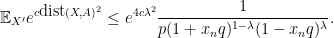
For 


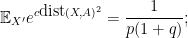
for 
![\displaystyle {\Bbb E}_{X} e^{c \hbox{dist}(X,A)^2} = \frac{1}{2} [ \frac{1}{p (1+q)} + e^{4 c \lambda^2} \frac{1}{p (1 - q)^{1-\lambda} (1 + q)^\lambda} ]](https://s0.wp.com/latex.php?latex=%5Cdisplaystyle+%7B%5CBbb+E%7D_%7BX%7D+e%5E%7Bc+%5Chbox%7Bdist%7D%28X%2CA%29%5E2%7D+%3D+%5Cfrac%7B1%7D%7B2%7D+%5B+%5Cfrac%7B1%7D%7Bp+%281%2Bq%29%7D+%2B+e%5E%7B4+c+%5Clambda%5E2%7D+%5Cfrac%7B1%7D%7Bp+%281+-+q%29%5E%7B1-%5Clambda%7D+%281+%2B+q%29%5E%5Clambda%7D+%5D&bg=ffffff&fg=000000&s=0&c=20201002)
so to establish (2), it suffices to pick

If 


Remark 3 Talagrand’s inequality is in fact far more general than this; it applies to arbitrary products of probability spaces, rather than just to
which are “locally certifiable” in the sense that whenever
is larger than some threshold
of coefficients of
which “certify” this fact (in the sense that
for any other
which agrees with
— 2. Gaussian concentration —
As mentioned earlier, there are analogous results when the uniform distribution on the cube
Proposition 3 (Gaussian concentration inequality) Let
for all
is a random Gaussian vector.
This inequality can be deduced from Lévy’s classical concentration of measure inequality for the sphere (with the optimal constant), but we will give an alternate proof due to Maurey and Pisier. It suffices to prove the following variant of Proposition 3:
Proposition 4 (Gaussian concentration inequality for Lipschitz functions) Let
be a function which is Lipschitz with constant
for all
. Then for any
for all
, where

Indeed, if one sets 


in either case. Also, since 

Now we prove Proposition 4. By the epsilon regularisation argument we may take 
for all 


We again use the exponential moment method. It suffices to show that
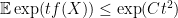
for some absolute constant 
Now we use a variant of the square and rearrange trick. Let 


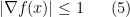
With an eye to exploiting (5), one might seek to use the fundamental theorem of calculus to write

But actually it turns out to be smarter to use a circular arc of integration, rather than a line segment:
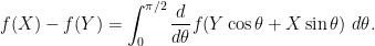
The reason for this is that 

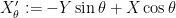
To exploit this, we first use Jensen’s inequality to bound

Applying the chain rule and taking expectations, we have

Let us condition 


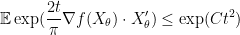
for some absolute constant

41 comments
Comments feed for this article
9 June, 2009 at 8:39 pm
student
Dear Prof Tao,
How do you pass from line segment integral to circular arc integral?
by change of variable ?
?
thanks
9 June, 2009 at 9:28 pm
Terence Tao
Dear student,
The circular arc identity is established directly from the fundamental theorem of calculus , rather than from applying a change of variables from the line segment identity (which doesn’t work). The point is that in higher dimensions, there are many inequivalent ways to apply the fundamental theorem of calculus to expand f(Y)-f(X) – one for each path from X to Y, and the key is to select the right one.
15 June, 2009 at 10:35 pm
student
Dear Prof. Tao,
I remember once you wrote that you will teach random matrix theory next semester. my request is that
Would you please start to post little by little some notes related to prerequisite material for that course? if we start to study during summer and get enough background it would be perfect for us.
thank you very much
16 June, 2009 at 7:10 am
Terence Tao
Actually, the class will be starting in the winter quarter (next January). I have not yet decided exactly what the topics will be, but apart from a basic graduate education in analysis, probability, linear algebra, and combinatorics it should be fairly self-contained.
16 June, 2009 at 11:59 am
Oded
One minor comment: the statement in Remark 2 seems almost vacuous. After all, the distance between *any* two points in {-1,+1}^n is at most 2\sqrt{n}. Maybe the correct behavior should be n^{1/4}?
16 June, 2009 at 12:25 pm
Terence Tao
Hmm, good point. On the other hand, the Azuma/McDiarmid argument also works if the metric is replaced by the much larger
  metric (although the mean or median of
  is somewhat harder to compute in that case). I’ll adjust the text to reflect this. (One could make the case that Talagrand’s inequality is to
  as Azuma’s inequality or McDiarmid’s inequality is to
  ; note the crucial use of Pythagoras’ theorem in the middle of the proof of Talagrand’s inequality.)
16 June, 2009 at 8:58 pm
vedadi
Dear Prof. Tao,
just after ” square and rearrange trick”, you say that you use Jensen’s inequality.
I guess your convex function is for
for 
in that case why do not we have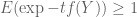 ?
?
Jensen’s ineq is , right?
thanks
16 June, 2009 at 9:16 pm
Terence Tao
Dear vedadi,
Yes, that was a typo, the expectation should be at least 1, rather than at most 1. (The subsequent inequalities did not have the typo, though.)
17 June, 2009 at 9:11 pm
student
Dear Prof Tao,
When we say ”let Y be an independent copy of X….” How do we guarantee the existence of that copy? Don’t we have some philosophical questions here too?
thanks
18 June, 2009 at 8:59 am
Terence Tao
Dear student,
Independent copies of a random variable can always be generated by the product measure construction,
http://en.wikipedia.org/wiki/Product_measure
This requires extending the underlying probability space to a finer one, but probability theory is designed in such a way that one can always do this without affecting any probabilistically meaningful quantities, such as probabilities of events or expectations, moments, correlations, and distributions of random variables. (As such, one of the guiding philosophies of probability theory is to not work with the underlying probability space if at all possible. The situation is somewhat analogous to differential geometry, which is designed to be invariant under changes of coordinates, and so the philosophy is often to avoid explicit manipulation of such coordinates whenever possible.)
Kallenberg’s “Foundations of modern probability” is a good reference for these sorts of foundational issues. However, it should be said that while such issues are of course important, especially from a philosophical or logical point of view, they rarely affect day-to-day usage of probability, much as the construction of the real numbers does not play a prominent role in real arithmetic, or as the construction of the Lebesgue integral does not play a prominent role in computation and estimation of integrals.
18 June, 2009 at 11:39 am
Anonymous
Dear Prof. Tao,
Could you please write a blog post on ”Large Deviation Principles” this summer by explaining the theory by examples and from your point of view?
thanks
2 July, 2009 at 6:05 am
ebrima saye
You are inspirational!!
2 July, 2009 at 7:57 pm
student
Dear Prof. Tao,
I could not find in which part I am doing a mistake in the following argument :
we know that if two random variables have the same distribution then their mean is the same. now
Let be a standard normal rv. and
  be an independent copy of it. then
  and
and  have the same distribution (?) but
 ![E[Z \cdot Z]=1](https://s0.wp.com/latex.php?latex=E%5BZ+%5Ccdot+Z%5D%3D1&bg=ffffff&fg=545454&s=0&c=20201002) and
and ![E[Z \cdot Z^{\prime}]=E[Z]E[Z^{\prime}]=0](https://s0.wp.com/latex.php?latex=E%5BZ+%5Ccdot+Z%5E%7B%5Cprime%7D%5D%3DE%5BZ%5DE%5BZ%5E%7B%5Cprime%7D%5D%3D0&bg=ffffff&fg=545454&s=0&c=20201002)
what is going on here?
thanks
3 July, 2009 at 7:58 am
Terence Tao
Dear student:
The same issue crops up if Z is a Bernoulli distribution (equal to +1 with probability 1/2, and -1 with probability -1/2). This example is elementary enough that you can work out everything from first principles; if you do so, you should see the error.
Dear Ben: X decomposes into two orthogonal components, PX and X-PX. X-PX is the orthogonal projection of X to V, so the distance from X to V is the length of PX. Since P is an orthogonal projection,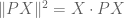 .
.
Alternatively, one can pick a coordinate system so that V is a coordinate plane, in which case all calculations can be done explicitly.
3 July, 2009 at 4:56 am
ben
Dear Prof Tao
could you explain why
thanks
5 July, 2009 at 3:33 pm
Anonymous
Dear Prof. Tao,
I did not see at which step you are using the independence of and
and 
and in the last paragraf, when you say ” let’s condition to be fixed….” do you mean you that you are using the following fact:
thanks
6 July, 2009 at 12:57 pm
Terence Tao
Yes, this is what is happening when one is conditioning on . The independence of
  and
and  is used precisely at this step, to ensure that
  retains its normal distribution even after conditioning on a fixed value of
  .
.
6 July, 2009 at 11:19 pm
lutfu
Dear Prof. Tao,
Let be two independent standart normal r.vs. then
since![E[\exp(X \cdot Y) | Y=t]=\exp(t^2/2)](https://s0.wp.com/latex.php?latex=E%5B%5Cexp%28X+%5Ccdot+Y%29+%7C+Y%3Dt%5D%3D%5Cexp%28t%5E2%2F2%29&bg=ffffff&fg=545454&s=0&c=20201002) we have
we have
is this argument true?
in which step we are using independence of and
and 
thanks
7 July, 2009 at 6:33 am
Terence Tao
Yes, this is correct. The independence is needed to establish the identity (because one needs X to remain normally distributed after conditioning on the event Y=t).
8 July, 2009 at 4:07 pm
lutfu
Dear Prof Tao,
Let be a seq of i.i.d. rvs. with mean zero.
as we know from as
as  the distribution of
Under the existence of second moment we know the limiting distribution of
my question is that do we know the distribution of
 for
for  under the suitable conditions? to which measure do they concentrate?
thanks
8 July, 2009 at 7:57 pm
Anonymous
Dear Prof. Tao,
Could you please give a proof for the Azuma-Hoeffding inequality?
thanks
3 January, 2010 at 10:22 pm
254A, Notes 1: Concentration of measure « What’s new
[…] by induction on dimension . In the case when are Bernoulli variables, this can be done; see this previous blog post. In the general case, it turns out that in order to close the induction properly, one must […]
5 January, 2010 at 4:20 pm
254A, Notes 0: A review of probability theory « What’s new
[…] by induction on dimension . In the case when are Bernoulli variables, this can be done; see this previous blog post. In the general case, it turns out that in order to close the induction properly, one must […]
13 June, 2010 at 1:23 pm
Laurent Jacques
Dear Terence,
Thank you for this verrry interesting post. I’d like to share with you some elements.
From what I know, Sub-Gaussian Random Variable (SGRV), such as Bernoulli RV, centered Uniform RV, Gaussian RV, … are defined as follows:
X is a SGRV if there exists one c>0 such that for all real value s,
E[ \exp (s X) ] <= exp (c^2 s^2/2)
See for instance V. V. Buldygin publications, e.g. "Sub-Gaussian random variables", doi:10.1007/BF01087176
If I'm not wrong, one interesting property of SBRV is that any linear combination of SGRV is SGRV with known characteristics. In particular, the "Gaussian standard", defined as the minimal "c" such that the definition above holds, behaves as the standard deviation of Gaussian RV with respect to linear combination of SGRV.
This implies also that if you rotate a sub-Gaussian random vector with iid SGRV components, you get also a sub-Gaussian random vector. The components of this latter are perhaps not iid anymore but at least they have all the same "Gaussian standard".
My question is thus the following:
**Do you think that Theorem 4 above could be easily generalized to sub-Gaussian random vectors of components with unit gaussian standard?**
It seems indeed that in many places in you proof, you use already key ingredients for this generalization:
* the sub-gaussian inequality definition;
* linear combinations (rotation) of Gaussian RVs which are themselves Gaussian.
Or perhaps this generalization is already known in the community (I didn't see it anyway in Talagrand/Ledoux's books)?
Best,
Laurent
18 August, 2010 at 12:43 am
Anonymous
Dear Prof. Tao
I have two questions about the proof for Proposition 4.
Firstly, It seems that there is a typo when you bound
exp(t(F(X)-F(Y))) by using Jensen Inequality, please check it if possible.
Secondly, the aim is
Eexp(tF(X))<=exp(Ct^2),
but the proof only tells us
Eexp(tF(X))<=exp(Ct),
Please give some explaination if possible.
Thanks.
[Corrected, thanks – T.]
20 August, 2010 at 2:50 am
Anonymous
Dear Prof. Tao
Have you checked the bound of exp(t(F(X)-F(Y))) in the proof of Proposition 4? There is still a typo in my opinion.
[Corrected, thanks – T.]
21 August, 2010 at 2:16 am
Anonymous
Dear Prof. Tao ? Some hints will be OK.
Can you tell me how to get
21 August, 2010 at 7:30 am
Terence Tao
If X is a Gaussian with mean zero and variance , then the moment generating function is
  , as can be seen by completing the square.
22 August, 2010 at 4:41 am
Anonymous
Dear Prof. Tao
I get it. Thanks for your reply. So far I have got a lot of interesting and useful mathemetical knowledge from your blog. Your earnest attitude and diligence impressed me. Thanks again.
16 November, 2010 at 10:04 pm
The Determinant of Random Bernoulli Matrices « Tsourolampis Blog
[…] [6] Talagrand’s inequality https://terrytao.wordpress.com/2009/06/09/talagrands-concentration-inequality/ […]
25 April, 2011 at 2:44 pm
Anonymous
Dear Prof. Tao,
is Talagrand concentration inequality still valid if we have independent but not identically distributed normally distributed component of ?
?
Thanks
8 May, 2012 at 1:15 am
Anonymous
Hi Professor Tao,
Does dist(X,V) = euclidean distance(X,V)?
Thanks.
[Yes – T.]
12 May, 2012 at 5:32 pm
sabyasachi chatterjee
Hello Professor Tao,
I have had to investigate the concentration of the log determinant of a matrix. Specifically, suppose M1,..Mk are random matrices p by p, iid from a given distribution(can assume that the entries of the matrix are bounded a.s or other regularity conds if needed) whose expected value is the identity matrix I. Now if I consider the matrix mean..(M1+…Mk)/k and look at its log determinant..will it concentrate around its mean? Will the mean go to zero as k go to infinity? Hence will it concentrate around 0? Is there any known result on this? Thanks
9 July, 2012 at 10:53 pm
mathepsilon
Does that mean, the small constant c in the gaussian concentration inequaltiy for lipschitz function is (pi^2)/8? Thank you! I really can not find this constant elsewhere.
10 July, 2012 at 9:08 am
Terence Tao
Well, the arguments given in the above post are not necessarily optimal; there may be other arguments that give a better value of c. (Note also that the value of c in Proposition 3 and Proposition 4 may differ, for instance the above arguments give a loss of a factor of 4 when passing from the latter to the former.)
I would try Ledoux’s book, as it has a number of proofs of this inequality and may discuss the question of optimal constants somewhere. (For instance, log-Sobolev methods tend to be quite sharp in general, and should yield good results in this case.)
17 December, 2013 at 2:11 pm
Anonymous
Dear Terry Tao,
can you get limit behavior of dist(X,V) (using Talagrand inequality or otherwise)?
Proposition 1 suggests that perhaps (after properly normalizing), the distribution of dist(X,V) converges to the normal distribution. Is it true?
I think it would nicely illustrate the strength of the presented method — similarly to the comparison of Chernoff bound and Central limit theorem.
Thanks,
Robert Samal
17 December, 2013 at 4:42 pm
Terence Tao
When X is a gaussian vector, then dist(X,V)^2 is a chi-squared distribution (with the number of degrees of freedom equal to the codimension of V), and so the central limit theorem shows that dist(X,V)^2 (and thus also dist(X,V)) is approximately gaussian when the codimension is large. For small codimension, one gets a chi distribution instead.
In the non-gaussian case, one can presumably get similar results either through a Lindeberg exchange argument, or through a central limit theorem for quadratic forms, although I don’t know if this has been done explicitly in the literature.
28 August, 2014 at 11:39 pm
Anonymous
Is proposition 4 valid for idd rvs with exponential moments?
12 September, 2015 at 2:46 pm
Anonymous
Small typo in props 3 and 4: n should be d (or vice versa)
[Corrected, thanks – T.]
15 December, 2018 at 4:53 pm
Ray
Dear Prof. Tao,
I am confused about some detail of the proof to proposition 2. How is defined when
  is an open set? And how is (4) defined if
  are empty sets?
Thanks!
15 December, 2018 at 8:41 pm
Ray
never mind, I realized that these details can be worked out and does not affect the proof.