Given a set  , a (simple) point process is a random subset
  of . (A non-simple point process would allow multiplicity; more formally, is no longer a subset of , but is a Radon measure on , where we give the structure of a locally compact Polish space, but I do not wish to dwell on these sorts of technical issues here.) Typically, will be finite or countable, even when is uncountable. Basic examples of point processes include
- (Bernoulli point process) is an at most countable set,
 is a parameter, and a random set such that the events
  for each
  are jointly independent and occur with a probability of
  each. This process is automatically simple.
- (Discrete Poisson point process) is an at most countable space,
 is a measure on (i.e. an assignment of a non-negative number
  to each ), and is a multiset where the multiplicity of
  in is a Poisson random variable with intensity , and the multiplicities of as varies in are jointly independent. This process is usually not simple.
- (Continuous Poisson point process) is a locally compact Polish space with a Radon measure , and for each
 of finite measure, the number of points
  that contains inside
  is a Poisson random variable with intensity
  . Furthermore, if
  are disjoint sets, then the random variables
  are jointly independent. (The fact that Poisson processes exist at all requires a non-trivial amount of measure theory, and will not be discussed here.) This process is almost surely simple iff all points in have measure zero.
- (Spectral point processes) The spectrum of a random matrix is a point process in
 (or in
  , if the random matrix is Hermitian). If the spectrum is almost surely simple, then the point process is almost surely simple. In a similar spirit, the zeroes of a random polynomial are also a point process.
A remarkable fact is that many natural (simple) point processes are determinantal processes. Very roughly speaking, this means that there exists a positive semi-definite kernel  such that, for any
  , the probability that
  all lie in the random set is proportional to the determinant
  . Examples of processes known to be determinantal include non-intersecting random walks, spectra of random matrix ensembles such as GUE, and zeroes of polynomials with gaussian coefficients.
I would be interested in finding a good explanation (even at the heuristic level) as to why determinantal processes are so prevalent in practice. I do have a very weak explanation, namely that determinantal processes obey a large number of rather pretty algebraic identities, and so it is plausible that any other process which has a very algebraic structure (in particular, any process involving gaussians, characteristic polynomials, etc.) would be connected in some way with determinantal processes. I’m not particularly satisfied with this explanation, but I thought I would at least describe some of these identities below to support this case. (This is partly for my own benefit, as I am trying to learn about these processes, particularly in connection with the spectral distribution of random matrices.) The material here is partly based on this survey of Hough, Krishnapur, Peres, and Virág.
— 1. Discrete determinantal processes —
In order to ignore all measure-theoretic distractions and focus on the algebraic structure of determinantal processes, we will first consider the discrete case when the space is just a finite set  of cardinality
  . We say that a process
  is a determinantal process with kernel
  , where is an
  symmetric real matrix, if one has

for all distinct  .
.
To build determinantal processes, let us first consider point processes of a fixed cardinality  , thus
  and is a random subset of of size , or in other words a random variable taking values in the set
  .
.
In this simple model, an -element point processes is basically just a collection of  probabilities
  , one for each
  , which are non-negative numbers which add up to
  . For instance, in the uniform point process where is drawn uniformly at random from
  , each of these probabilities
  would equal
  . How would one generate other interesting examples of -element point processes?
For this, we can borrow the idea from quantum mechanics that probabilities can arise as the square of coefficients of unit vectors, though unlike quantum mechanics it will be slightly more convenient here to work with real vectors rather than complex ones. To formalise this, we work with the  exterior power
  of the Euclidean space
  ; this space is sort of a “quantisation” of , and is analogous to the space of quantum states of identical fermions, if each fermion can exist classically in one of
  states (or “spins”). (The requirement that the process be simple is then analogous to the Pauli exclusion principle.)
This space of -vectors in is spanned by the wedge products  with
with  , where
  is the standard basis of . There is a natural inner product to place on by declaring all the to be orthonormal.
Lemma 1 If  is any orthonormal basis of , then the
  for are an orthonormal basis for .
Proof: By definition, this is true when  . If the claim is true for some orthonormal basis , it is not hard to see that the claim also holds if one rotates
  and
and  in the plane that they span by some angle
  , where
  are arbitrary. But any orthonormal basis can be rotated into any other by a sequence of such rotations (e.g. by using Euler angles), and the claim follows.
Corollary 2 If  are vectors in , then the magnitude of
  is equal to the -dimensional volume of the parallelopiped spanned by .
Proof: Observe that applying row operations to  (i.e. modifying one by a scalar multiple of another
  ) does not affect either the wedge product or the volume of the parallelopiped. Thus by using the Gram-Schmidt process, we may assume that the are orthogonal; by normalising we may assume they are orthonormal. The claim now follows from the preceding lemma.
From this and the ordinary Pythagorean theorem in the inner product space , we conclude the multidimensional Pythagorean theorem: the square of the -dimensional volume of a parallelopiped in is the sum of squares of the -dimensional volumes of the projection of that parallelopiped to each of the coordinate subspaces  . (I believe this theorem was first observed in this generality by Donchian and Coxeter.) We also note another related fact:
Lemma 3 (Gram identity) If are vectors in , then the square of the magnitude of is equal to the determinant of the Gram matrix  .
.
Proof: Again, the statement is invariant under row operations, and one can reduce as before to the case of an orthonormal set, in which case the claim is clear. (Alternatively, one can proceed via the Cauchy-Binet formula.)
If we define  , then we have identified the standard basis of with by identifying
  with
with  . As a consequence of this and the multidimensional Pythagorean theorem, every unit -vector
  in determines an -element point process on , by declaring the probability of taking the value to equal
  for each . Note that multiple -vectors can generate the same point process, because only the magnitude of the coefficients
  are of interest; in particular, and
  generate the same point process. (This is analogous to how multiplying the wave function in quantum mechanics by a complex phase has no effect on any physical observable.)
Now we can introduce determinantal processes. If  is an -dimensional subspace of , we can define the (projection) determinantal process
  associated to to be the point process associated to the volume form of , i.e. to the wedge product of an orthonormal basis of . (This volume form is only determined up to sign, because the orientation of has not been fixed, but as observed previously, the sign of the form has no impact on the resulting point process.)
By construction, the probability that the point process is equal to a set  is equal to the square of the determinant of the
  matrix consisting of the
  coordinates of an arbitrary orthonormal basis of . By extending such an orthonormal basis to the rest of , and representing
  in this basis, it is not hard to see that
  can be interpreted geometrically as the square of the volume of the parallelopiped generated by
  , where
  is the orthogonal projection onto .
In fact we have the more general fact:
Lemma 4 If  and
and  are distinct elements of , then
  is equal to the square of the
  -dimensional volume of the parallelopiped generated by the orthogonal projections of
  to .
to .
Proof: We can assume that  , since both expressions in the lemma vanish otherwise.
By (anti-)symmetry we may assume that  . By the Gram-Schmidt process we can find an orthonormal basis of such that each is orthogonal to
  .
.
Now consider the  matrix
  with rows , thus vanishes below the diagonal. The probability
  is equal to the sum of squares of the determinants of all the minors of that contain the first rows. As vanishes below the diagonal, we see from cofactor expansion that this is equal to the product of the squares of the first diagonal entries, times the sum of squares of the determinants of all the
  minors of the bottom
  rows. But by the generalised Pythagorean theorem, this latter factor is the square of the volume of the parallelopiped generated by
  , which is . Meanwhile, by the base times height formula, we see that the product of the first diagonal entries of is equal in magnitude to the -dimensional volume of the orthogonal projections of
  to . The claim follows.
In particular, we have  for any
  . In particular, if
  lies in , then almost surely lies in , and when is orthogonal to , almost surely is disjoint from .
Let  denote the matrix coefficients of the orthogonal projection . From Lemma 4 and the Gram identity, we conclude that is a determinantal process (see (1)) with kernel . Also, by combining Lemma 4 with the generalised Pythagorean theorem, we conclude a monotonicity property:
Lemma 5 (Monotonicity property) If  are nested subspaces of , then
  for every
  .
.
This seems to suggest that there is some way of representing  as the union of
  with another process coupled with , but I was not able to build a non-artificial example of such a representation. On the other hand, if
  and
and  , then the process
  associated with the direct sum
  has the same distribution of the disjoint union of with an independent copy of
  .
.
The determinantal process interacts nicely with complements:
Lemma 6 (Hodge duality) Let be an -dimensional subspace of . The  -element determinantal process
  associated to the orthogonal complement
  of has the same distribution as the complement
  of the -element determinantal process associated to .
Proof: We need to show that  for all
  . By symmetry we can take
  . Let and
  be an orthonormal basis for and respectively, and let be the resulting
  orthogonal matrix; then the task is to show that the top minor
  of has the same determinant squared as the bottom
  minor
minor  . But if one splits
  , we see from the orthogonality property that
  and
and  , where
  is the identity matrix. But from the singular value decomposition we see that
  and
and  have the same determinant, and the claim follows. (One can also establish this lemma using the Hodge star operation.)
From this lemma we see that  is a determinantal process with kernel
  . In particular, we have

The construction of the determinantal process given above is somewhat indirect. A more direct way to build the process exploits the following lemma:
Lemma 7 Let be an -dimensional subspace of , let be the corresponding -element determinantal process, and let  for some
  . Then the if one conditions on the event that
  (assuming this event has non-zero probability), the resulting -element process
  has the same distribution as the -element determinantal process associated to the -dimensional subspace
  of that is orthogonal to
  .
.
Proof: By symmetry it suffices to consider the case  . By a further application of symmetry it suffices to show that

By the Gram-Schmidt process, we can find an orthonormal basis of whose matrix of coefficients vanishes below the diagonal. One then easily verifies (using Lemma 4) that  is the product of the diagonal entries,
  is the product of the first , and
  is the product of the last , and the claim follows.
From this lemma, it is not difficult to see that one can build recursively as  , where
  is a random variable drawn from with a
  for each , and
  is the subspace of orthogonal to
  . Another consequence of this lemma and the monotonicity property is the negative dependence inequality

for any disjoint  ; thus the presence of on one set
  reduces the chance of being present on a disjoint set
  (not surprising, since has fixed size).
Thus far, we have only considered point processes with a fixed number of points. As a consequence, the determinantal kernel involved here is of a special form, namely the coefficients of an orthogonal projection matrix to an -dimensional space (or equivalently, a symmetric matrix whose eigenvalues consist of ones and zeroes). But one can create more general point processes by taking a mixture of the fixed-number processes, e.g. first picking a projection kernel (or a subspace ) by some random process, and then sampling from the point process associated to that kernel or subspace.
For instance, let  be an orthonormal basis of , and let
  be weights. Then we can create a random subspace of by setting equal to the span
  of some random subset
  of the basis
  , where each
  lies in
  with an independent probability of
  , and then sampling from . Then will be a point process whose cardinality can range from
  to . Given any set
  , we can then compute the probability
  as
as

where is selected as above. Using (1), we have

But  , where
  is the
  coordinate of
  . Thus we can write
where  is the indicator of the event
  , and
, and  is the rank one matrix
  . Using multilinearity of the determinant, and the fact that any determinant involving two or more rows of the same rank one matrix automatically vanishes, we see that we can express

wheree  is the matrix whose first row is the same as that of
  , the second row is the same as that of
  , and so forth. Taking expectations in , the quantity
  becomes
  . Undoing the multilinearity step, we conclude that

and thus is a determinantal process with kernel

To summarise, we have created a determinantal process whose kernel is now an arbitrary symmetric matrix with eigenvalues ![{\lambda_1,\ldots,\lambda_n \in [0,1]}](https://s0.wp.com/latex.php?latex=%7B%5Clambda_1%2C%5Cldots%2C%5Clambda_n+%5Cin+%5B0%2C1%5D%7D&bg=ffffff&fg=000000&s=0&c=20201002) , and it is a mixture of constant-size processes
, and it is a mixture of constant-size processes  . In particular, the cardinality
  of this process has the same distribution as the cardinality
  of the random subset of
  , or in other words
  , where
  are independent Bernoulli variables with expectation
  respectively.
Observe that if one takes a determinantal process with kernel , and restricts it to a subset  of , then the resulting process
  is a determinantal process whose kernel
  is simply the restriction of to the
  block of
  . Applying the previous observation, we conclude that the random variable
  has the same distribution as the sum of
  independent Bernoulli variables, whose expectations are the eigenvalues of the restriction of to . (Compare this to the Poisson point process with some intensity measure , where the distribution of is a Poisson process with intensity .) Note that most point processes do not obey this property (e.g. the uniform distribution on does not unless
  or
or  ), and so most point processes are not determinantal.
It is known that increasing a positive semi-definite matrix by another positive semi-definite matrix does not decrease the determinant (indeed, it does not decrease any eigenvalue, by the minimax characterisation of those eigenvalues). As a consequence, if the kernel of a determinantal process  is larger than the kernel of another determinantal process in the sense that
  is positive semi-definite, then is “larger” than in the sense that
  for all . A particularly nice special case is when
  for some
  , then
  for all , and one can interpret as the process obtained from by deleting each element of independently at random with probability
  (i.e. keeping that element independently at random with probability
  ).
).
As a consequence of this, one can obtain a converse to our previous construction of determinantal processes, and conclude that a determinantal process can be associated to a symmetric kernel only if the eigenvalues of lie between zero and one. The fact that is positive semi-definite follows from the fact that all symmetric minors of have non-negative determinant (thanks to (1)). Now suppose for contradiction that has an eigenvalue larger than , then one can find  such that the largest eigenvalue of
  is exactly . By our previous discussion, the process
  associated to is then formed from the process
  by deleting each element of with non-zero probability; in particular, is empty with non-zero probability. On the other hand, we know that
  has the distribution of the sum of independent Bernoulli variables, at least one of which is with probability one, a contradiction. (This proof is due to Hough et al., though the result is originally due to Soshnikov. An alternate proof is to extend the identity (2) to all determinantal processes and conclude that
  is necessarily positive definite.)
— 2. Continuous determinantal processes —
One can extend the theory of discrete determinantal processes to the continuous setting. For simplicity we restrict attention to (simple) point processes  on the real line. A process is said to have correlation functions
  for if the
  are symmetric, non-negative, and locally integrable, and one has the formula

for any bounded measurable symmetric  with compact support, where the left-hand side is summed over all -tuples of distinct points in (this sum is of course empty if
  ). Intuitively, the probability that contains an element in the infinitesimal interval
 ![{[x_i,x_i+dx_i]}](https://s0.wp.com/latex.php?latex=%7B%5Bx_i%2Cx_i%2Bdx_i%5D%7D&bg=ffffff&fg=000000&s=0&c=20201002) for all
for all  and distinct
  is equal to
  . The are not quite probability distributions; instead, the integral
  is equal to
  . Thus, for instance, if is a constant-size process of cardinality , then has integral
  on
on  for and vanishes for
  .
.
If the correlation functions exist, it is easy to see that they are unique (up to almost everywhere equivalence), and can be used to compute various statistics of the process. For instance, an application of the inclusion-exclusion principle shows that for any bounded measurable set , the probability that  is (formally) equal to

A process is determinantal with some symmetric measurable kernel  if it has correlation functions given by the formula

Informally, the probability that intersects the infinitesimal intervals for distinct is  . (Thus, is most naturally interpreted as a half-density, or as an integral operator from
  to .)
to .)
There are analogues of the discrete theory in this continuous setting. For instance, one can show that a symmetric measurable kernel generates a determinantal process if and only if the associated integral operator  has spectrum lies in the interval
 ![{[0,1]}](https://s0.wp.com/latex.php?latex=%7B%5B0%2C1%5D%7D&bg=ffffff&fg=000000&s=0&c=20201002) . The analogue of (2) is the formula
. The analogue of (2) is the formula

more generally, the distribution of is the sum of independent Bernoulli variables, whose expectations are the eigenvalues of  . Finally, if is an orthogonal projection onto an -dimensional space, then the process has a constant size of . Conversely, if is a process of constant size , whose correlation function
  is given by (3), where is an orthogonal projection onto an -dimensional space, then (3) holds for all other values of as well, and so is a determinantal process with kernel . (This is roughly the analogue of Lemma 4.)
These facts can be established either by approximating a continuous process as the limit of discrete ones, or by obtaining alternate proofs of several of the facts in the previous section which do not rely as heavily on the discrete hypotheses. See Hough et al. for details.
A Poisson process can be viewed as the limiting case of a determinantal process in which degenerates to a (normalisation of) a multiplication operator  , where is the intensity function.
— 3. The spectrum of GUE —
Now we turn to a specific example of a continuous point process, namely the spectrum  of the Gaussian unitary ensemble
  , where the
  are independent for
  with mean zero and variance , with being the standard complex gaussian for
  and the standard real gaussian
  for
for  . The probability distribution of
  can be expressed as
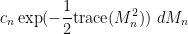
where  is Lebesgue measure on the space of Hermitian matrices, and
  is some explicit normalising constant.
The -point correlation function of can be computed explicitly:
Lemma 8 (Ginibre formula) The -point correlation function of the GUE spectrum is given by
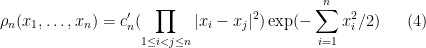
where the normalising constant  is chosen so that
  has integral .
The constant  is essentially the reciprocal of the partition function for this ensemble, and can be computed explicitly, but we will not do so here.
Proof: Let  be a diagonal random matrix
  whose entries are drawn using the distribution defined by (4), and let
  be a unitary matrix drawn uniformly at random (with respect to Haar measure on
  ) and independently of . It will suffice to show that the GUE has the same probability distribution as
  . Since probability distributions have total mass one, it suffices to show that their distributions differ up to multiplicative constants.
The distributions of and are easily seen to be continuous and invariant under unitary rotations. Thus, it will suffice to show that their probability density at a given diagonal matrix  are the same up to multiplicative constants. We may assume that the
  are distinct, since this occurs for almost every choice of
  .
.
On the one hand, the probability density of at is proportional to  . On the other hand, a short computation shows that if
  is within a distance
  of for some infinitesimal
  , then (up to permutations) must be a distance from , and the
  entry of
  must be a complex number of size
  for , while the diagonal entries of can be arbitrary phases. Pursuing this computation more rigorously (e.g. using the Harish-Chandra formula) and sending
  , one can show that the probability density of at is a constant multiple of
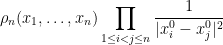
(the square here arising because of the complex nature of the coefficient of ) and the claim follows.
One can also represent the -point correlation functions as a determinant:
Lemma 9 (Gaudin-Mehta formula) The -point correlation function  of the GUE spectrum is given by

where  is the kernel of the orthogonal projection in to the space spanned by the polynomials
  for
for  . In other words, is the -point determinantal process with kernel
  .
.
Proof: By the material in the preceding section, it suffices to establish this for  . As is the kernel of an orthogonal projection to an -dimensional space, it generates an -point determinantal process and so
  has integral
  . Thus it will suffice to show that and agree up to multiplicative constants.
By Gram-Schmidt, one can find an orthonormal basis  , for the range of , with each
  a polynomial of degree (these are essentially the Hermite polynomials). Then we can write

Cofactor expansion then shows that is equal to  times a polynomial
  in of degree at most
  . On the other hand, this determinant is always non-negative, and vanishes whenever
  for any , and so must contain
  as a factor for all . As the total degree of all these (relatively prime) factors is
  , the claim follows.
This formula can be used to obtain asymptotics for the (renormalised) GUE eigenvalue spacings in the limit  , by using asymptotics for (renormalised) Hermite polynomials; this was first established by Dyson.


29 comments
Comments feed for this article
23 August, 2009 at 1:29 pm
Anonymous
Dear Prof. Tao,
before is
is 
 or
or  ?
?
thanks
[Corrected, thanks]
23 August, 2009 at 2:43 pm
Anonymous
Is the expository tag missing? [Added, thanks.]
24 August, 2009 at 9:20 am
Craig Tracy
TASEP (=totally asymmetric simple exclusion process) is a determinantal process (see Kurt Johansson’s paper “Shape Fluctuations and Random Matrices”) but the more general ASEP (=asymmetric simple exclusion process) is, as far as I understand, not a determinantal process. However, in recent work with Harold Widom we have shown that the limit laws for ASEP are the same as for TASEP (see http://arxiv.org/a/tracy_c_1.atom) thus establishing “KPZ universality”. Hence, what is proved at the level of determinantal processes appears to extend to a larger class of processes. This is similar in spirit to the Soshnikov/Tao/Vu work on Wigner matrices.
24 August, 2009 at 9:35 am
ramanujantao
What is the point of writing “$la tex {x \in A}$ instead of ”$la tex x \in A$?”
24 August, 2009 at 4:10 pm
ateixeira
The LateX code appear between {} because of Luca Trevisan’s LateX to wordpress converter: http://lucatrevisan.wordpress.com/latex-to-wordpress/
It is pretty handy if one is writing long posts that use a lot of mathematical expressions in WordPress.
24 August, 2009 at 10:08 am
carnegie
Dear Professor Tao,
There seems to be a deep link between determinantal processes, random matrix theory, orthogonal polynomials, and integrable systems. Your previous commenter Craig Tracy has done very pioneering work in all these areas.
It would be interesting to know if the determinants which appear are related to the determinants involved in the Kyoto school’s approach to quantum field theory. Determinants there appear essentially when considering changes of basis in a Grassmannian.
24 August, 2009 at 10:26 pm
From Helly to Cayley IV: Probability « Combinatorics and more
[…] of studying determinental probability measures. (You can read more about determinental processes in this post of Terry Tao, and this survey paper by J. Ben Hough, Manjunath Krishnapur, Yuval Peres, and Bálint […]
25 August, 2009 at 1:19 am
Gil Kalai
Dear Terry, It is very cool how the algebra gives quick proofs and insights to these issues. Is the following known: start with a random Gausian n by n matrix and consider the associated (latex 2^n\times 2^n$) random matrix on the entire exterior algebra. What is the distribution of the eigenvalues of the huge matrix (and the distribution of spacing; maximual eigenvalue etc.) One can simply talk about the set of all products of eigenvalues but maybe the algebraic setting may help.
7 September, 2009 at 3:25 am
Gil Kalai
Let me add that Gerard Letac and Wlodzimiers Btyc have considered the distribution of eigenvalues of compund matrices.
My motivation was related toa polymath4 discussion: if the eigenvalues are analogous to the primes then the eigenvalues of the huge matrix are analogous to the squre free integers. Maybe in some sense and for some appropriate normalization (the normalization is important) the
  eigenvalues of the huge matrix will behave like a poisson point process (e.g. in terms of spacings joint-distribution).
Of course (as Gerard pointed) when you create 2^n numbers out of n you lose a lot of randomness but still for local property (like spacing distributions) you may recover a behavior of Poisson point process for the huge matrix while the behavior for the small matrix is very different.
25 August, 2009 at 3:31 pm
Anonymous
Dear Prof. Tao,
what do you mean by ”Lebesgue measure on the space of Hermitian matrices….” ?
do not we have Lebesque measure just on ?
?
thanks
26 August, 2009 at 9:38 am
JC
The space of hermitian matrices forms a real vector space (of dimension ), so Lebesgue measure is defined.
26 August, 2009 at 12:48 pm
Anonymous
thanks for the answer
26 August, 2009 at 11:33 am
On the geometric meaning of the Cauchy Schwarz inequality, an intro to exterior powers, and surface integrals « A Day in the Life of a Wild Positron
[…] the meantime, check out this post of Terence Tao on how this same induced inner product can be used to construct interesting processes […]
27 August, 2009 at 10:24 pm
Manju
Dear Terry, a possibly related question to understanding why so many processes are determinantal is about how to check if a process is determinantal? If they are so prevalent there ought to be a simple way, but we only know to do this by computing all correlations. Any light on this would be helpful.
By the way, the exterior algebra formulation is similar to Russell Lyons’ paper
http://front.math.ucdavis.edu/0204.5325. And a longer version (with examples) of our survey is now available in two chapters of
Click to access GAF_book.pdf
4 September, 2009 at 3:17 pm
Russell Lyons
Hi, Terry.
You write:
This seems to suggest that there is some way of representing {A_W} as the union of {A_V} with another process coupled with {A_V}, but I was not able to build a non-artificial example of such a representation.
I’m not sure what that means, but in my paper (mentioned by Manju and cited by Hough et al), I do prove this is always possible. There are other questions about couplings that are open, though, especially for more than two processes. I’d be very interested to see progress on any of them.
Best,
Russ
4 September, 2009 at 3:41 pm
Terence Tao
Thanks Russ! I assume you are referring to Theorem 6.2 of your paper (which generalises Lemma 5 here). I agree that there exists a way to couple A_V to A_W in such a way that the former set is always a subset of the latter, but I guess I was looking for some sort of “canonical” or “explicit” construction of such a coupling, possibly with additional nice properties (e.g. perhaps one could arrange so that the difference was also a determinantal process, e.g. associated to the orthogonal complement of V in W? But perhaps this is too naive). [Added later: It seems that
  from Pythagoras’ theorem, which is some weak evidence in favour of such a coupling existing.]
[Added yet later: It seems that you raise a similar question in page 38 of your paper. Actually this seems to be an interesting question; I think I will add it to the list of potential polymath projects for the future.]
4 September, 2009 at 5:20 pm
Russell Lyons
Yes, I was referring to my Thm 6.2 and Question 10.1. I have tested this question on numerous random instances up to dimension 9. A coupling always seems to exist, though, of course, I know nothing about a natural coupling. See also the questions about complete couplings in the following section, which I have also tested somewhat.
17 November, 2009 at 4:06 pm
The Lindstrom-Gessel-Viennot lemma « Annoying Precision
[…] lemma implies that non-intersecting random walks are a determinantal process, which connects them to many other mysterious processes. I wish I knew what to make of […]
1 January, 2010 at 8:47 pm
254A, Notes 0: A review of probability theory « What’s new
[…] of eigenvalues (counting multiplicity) of a random matrix . I discuss point processes further in this previous blog post. We will return to point processes (and define them more formally) later in this course. Remark 2 […]
23 February, 2010 at 10:03 pm
254A, Notes 6: Gaussian ensembles « What’s new
[…] Remark 5 This remarkable identity is part of the beautiful algebraic theory of determinantal processes, which I discuss further in this blog post. […]
24 August, 2010 at 11:54 pm
Roozbeh
Dear Terry, it seems there is a crucial flaw in proof of lemma 6 (Hodge duality). the correct formula is Y*Y= I – W*W not Y*Y= I – Z*Z.
I have seen a explicit form of K(x,y) in lemma 9, it would be nice if you could guide me to see their equivalence.
at the end, I have to say your notes are the best among similar notes, I’m writing my graduate thesis manly based on your notes.
25 August, 2010 at 8:02 am
Terence Tao
I believe the formula is correct as it stands (it comes from
  ). You may be thinking instead of the formula
  , which comes from
  .
.
I discuss the Gaudin kernel further in these notes:
21 December, 2010 at 1:51 pm
The mesoscopic structure of GUE eigenvalues « What’s new
[…] whenever are and matrices respectively (or more generally, and could be linear operators with sufficiently good spectral properties that make both sides equal). Note that the left-hand side is an determinant, while the right-hand side is a determinant; this formula is particularly useful when computing determinants of large matrices (or of operators), as one can often use it to transform such determinants into much smaller determinants. In particular, the asymptotic behaviour of determinants as can be converted via this formula to determinants of a fixed size (independent of ), which is often a more favourable situation to analyse. Unsurprisingly, this trick is particularly useful for understanding the asymptotic behaviour of determinantal processes. […]
7 March, 2012 at 10:18 pm
The asymptotic distribution of a single eigenvalue gap of a Wigner matrix « What’s new
[…] decoupled from the event in (1) when is drawn from GUE. To do this we use some of the theory of determinantal processes, and in particular the nice fact that when one conditions a determinantal process to the event that […]
22 October, 2013 at 1:44 pm
jsteinhardt
The separate construction of a general DPP as a mixture of fixed-size DPPs seems a bit unsatisfying; could we try to write the general construction directly in terms of exterior powers as follows?
Associate the exterior algebra with the corresponding (anti-commutative) polynomial algebra. Then the fixed-size DPP construction is obtained by taking to be orthonormal degree-1 (linear) polynomials and letting
  . Since
  is homogeneous of degree
  , the DPP is fixed-size. But we could instead imagine taking
  to be *affine* polynomials, in which case
  is inhomogeneous but will still satisfy
  as long as the
  are orthonormal. Does this work or am I missing something?
Thanks,
Jacob
22 October, 2013 at 2:07 pm
Russell Lyons
Jacob,
I could not figure out what you are saying in a way that makes it work. However, I can say that the general case arises from the fixed-size case just by restricting to a subset of the ground set. See Sec. 8 of my paper referred to above.
–Russ
22 October, 2013 at 3:17 pm
Terence Tao
Yes, I think this works, although one has to interpret the orthonormality of properly (it seems that only the vector parts of the
  are orthogonal to each other). Namely, to obtain a determinantal process with kernel
  for some orthonormal system
  , we set
  to be the sum
  of a scalar and a vector, and then I believe that the magnitude square of the components of the wedge product
  give the distribution of the point process.
23 March, 2014 at 9:49 pm
Quora
What are the most unexpected places you’ve seen determinants come up?
Thanks for the great answer, Justin. My first exposure to DPPs came from Terence Tao’s blog (which I found really helpful as a precursor to 1207.6083): https://terrytao.wordpress.com/2009/08/23/determinantal-processes/
18 June, 2015 at 11:10 pm
Entropy optimality: Forster’s isotropy | tcs math
[…] of entropy optimality applied to a determinental measure (see, for instance, Terry Tao’s post on determinental processes). I think this is an especially fertile setting for entropy maximization, but this will be the only […]