Our study of random matrices, to date, has focused on somewhat general ensembles, such as iid random matrices or Wigner random matrices, in which the distribution of the individual entries of the matrices was essentially arbitrary (as long as certain moments, such as the mean and variance, were normalised). In these notes, we now focus on two much more special, and much more symmetric, ensembles:
- The Gaussian Unitary Ensemble (GUE), which is an ensemble of random
 Hermitian matrices
  in which the upper-triangular entries are iid with distribution
  , and the diagonal entries are iid with distribution
  , and independent of the upper-triangular ones; and
- The Gaussian random matrix ensemble, which is an ensemble of random (non-Hermitian) matrices whose entries are iid with distribution .
The symmetric nature of these ensembles will allow us to compute the spectral distribution by exact algebraic means, revealing a surprising connection with orthogonal polynomials and with determinantal processes. This will, for instance, recover the semi-circular law for GUE, but will also reveal fine spacing information, such as the distribution of the gap between adjacent eigenvalues, which is largely out of reach of tools such as the Stieltjes transform method and the moment method (although the moment method, with some effort, is able to control the extreme edges of the spectrum).
Similarly, we will see for the first time the circular law for eigenvalues of non-Hermitian matrices.
There are a number of other highly symmetric ensembles which can also be treated by the same methods, most notably the Gaussian Orthogonal Ensemble (GOE) and the Gaussian Symplectic Ensemble (GSE). However, for simplicity we shall focus just on the above two ensembles. For a systematic treatment of these ensembles, see the text by Deift.
— 1. The spectrum of GUE —
We have already shown using Dyson Brownian motion in Notes 3b that we have the Ginibre formula

for the density function of the eigenvalues  of a GUE matrix , where

is the Vandermonde determinant. We now give an alternate proof of this result (omitting the exact value of the normalising constant  ) that exploits unitary invariance and the change of variables formula (the latter of which we shall do from first principles). The one thing to be careful about is that one has to somehow quotient out by the invariances of the problem before being able to apply the change of variables formula.
One approach here would be to artificially “fix a gauge” and work on some slice of the parameter space which is “transverse” to all the symmetries. With such an approach, one can use the classical change of variables formula. While this can certainly be done, we shall adopt a more “gauge-invariant” approach and carry the various invariances with us throughout the computation. (For a comparison of the two approaches, see this previous blog post.)
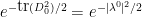
We turn to the details. Let  be the space of Hermitian matrices, then the distribution
  of a GUE matrix is a absolutely continuous probability measure on , which can be written using the definition of GUE as
where  is Lebesgue measure on
  ,
,  are the coordinates of , and
  is a normalisation constant (the exact value of which depends on how one normalises Lebesgue measure on ). We can express this more compactly as

Expressed this way, it is clear that the GUE ensemble is invariant under conjugations  by any unitary matrix.
Let  be the diagonal matrix whose entries
  are the eigenvalues of in descending order. Then we have
  for some unitary matrix
  . The matirx
  is not uniquely determined; if
  is diagonal unitary matrix, then commutes with , and so one can freely replace with
  . On the other hand, if the eigenvalues of
  are simple, then the diagonal matrices are the only matrices that commute with , and so this freedom to right-multiply by diagonal unitaries is the only failure of uniqueness here. And in any case, from the unitary invariance of GUE, we see that even after conditioning on , we may assume without loss of generality that is drawn from the invariant Haar measure on
  . In particular, and can be taken to be independent.
Fix a diagonal matrix 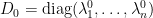 for some
  , let
, let  be extremely small, and let us compute the probability

that lies within  of
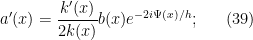
of  in the Frobenius norm. On the one hand, the probability density of is proportional to
near (where we write  ) and the volume of a ball of radius in the
  -dimensional space is proportional to
  , so (2) is equal to

for some constant  depending only on
  , where
  goes to zero as
  (keeping and fixed). On the other hand, if
  , then by the Weyl inequality (or Hoffman-Weilandt inequality) we have
  (we allow implied constants here to depend on and on ). This implies
  , thus
  . As a consequence we see that the off-diagonal elements of are of size
  . We can thus use the inverse function theorem in this local region of parameter space and make the ansatz

where  is a bounded diagonal matrix, is a diagonal unitary matrix, and
  is a bounded skew-adjoint matrix with zero diagonal. (Note here the emergence of the freedom to right-multiply by diagonal unitaries.) Note that the map
  has a non-degenerate Jacobian, so the inverse function theorem applies to uniquely specify
  (and thus ) from
  in this local region of parameter space.
Conversely, if  take the above form, then we can Taylor expand and conclude that

and so

We can thus bound (2) from above and below by expressions of the form

As is distributed using Haar measure on , is (locally) distributed using  times a constant multiple of Lebesgue measure on the space
  of skew-adjoint matrices with zero diagonal, which has dimension
  . Meanwhile, is distributed using
  times Lebesgue measure on the space of diagonal elements. Thus we can rewrite (4) as
where  and
and  denote Lebesgue measure and
  depends only on .
Observe that the map 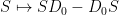 dilates the (complex-valued)
  entry of by
  , and so the Jacobian of this map is
  . Applying the change of variables, we can express the above as
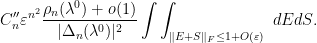
The integral here is of the form  for some other constant
  . Comparing this formula with (3) we see that

for yet another constant  . Sending we recover an exact formula

when  is simple. Since almost all Hermitian matrices have simple spectrum (see Exercise 10 of Notes 3a), this gives the full spectral distribution of GUE, except for the issue of the unspecified constant.
Remark 1 In principle, this method should also recover the explicit normalising constant  in (1), but to do this it appears one needs to understand the volume of the fundamental domain of with respect to the logarithm map, or equivalently to understand the volume of the unit ball of Hermitian matrices in the operator norm. I do not know of a simple way to compute this quantity (though it can be inferred from (1) and the above analysis). One can also recover the normalising constant through the machinery of determinantal processes, see below.
Remark 2 The above computation can be generalised to other -conjugation-invariant ensembles whose probability distribution is of the form

for some potential function  (where we use the spectral theorem to define
  ), yielding a density function for the spectrum of the form

Given suitable regularity conditions on , one can then generalise many of the arguments in these notes to such ensembles. See this book by Deift for details.
— 2. The spectrum of gaussian matrices —
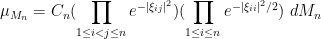
The above method also works for gaussian matrices  , as was first observed by Dyson (though the final formula was first obtained by Ginibre, using a different method). Here, the density function is given by

where  is a constant and
  is Lebesgue measure on the space
  of all complex matrices. This is invariant under both left and right multiplication by unitary matrices, so in particular is invariant under unitary conjugations as before.
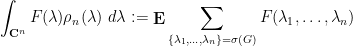
This matrix has complex (generalised) eigenvalues 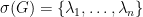 , which are usually distinct:
Exercise 3 Let  . Show that the space of matrices in with a repeated eigenvalue has codimension
  .
.
Unlike the Hermitian situation, though, there is no natural way to order these complex eigenvalues. We will thus consider all  possible permutations at once, and define the spectral density function
  of by duality and the formula
for all test functions  . By the Riesz representation theorem, this uniquely defines
  (as a distribution, at least), although the total mass of is rather than
  due to the ambiguity in the spectrum.
Now we compute (up to constants). In the Hermitian case, the key was to use the factorisation  . This particular factorisation is of course unavailable in the non-Hermitian case. However, if the non-Hermitian matrix has simple spectrum, it can always be factored instead as
  , where is unitary and
  is upper triangular. Indeed, if one applies the Gram-Schmidt process to the eigenvectors of and uses the resulting orthonormal basis to form , one easily verifies the desired factorisation. Note that the eigenvalues of are the same as those of , which in turn are just the diagonal entries of .
Exercise 4 Show that this factorisation is also available when there are repeated eigenvalues. (Hint: use the Jordan normal form.)
To use this factorisation, we first have to understand how unique it is, at least in the generic case when there are no repeated eigenvalues. As noted above, if , then the diagonal entries of form the same set as the eigenvalues of .
Now suppose we fix the diagonal  of , which amounts to picking an ordering of the eigenvalues of . The eigenvalues of are , and furthermore for each
  , the eigenvector of associated to
  lies in the span of the last
  basis vectors
  of
of  , with a non-zero
  coefficient (as can be seen by Gaussian elimination or Cramer’s rule). As
  with unitary, we conclude that for each , the
  column of lies in the span of the eigenvectors associated to
  . As these columns are orthonormal, they must thus arise from applying the Gram-Schmidt process to these eigenvectors (as discussed earlier). This argument also shows that once the diagonal entries of are fixed, each column of is determined up to rotation by a unit phase. In other words, the only remaining freedom is to replace by for some unit diagonal matrix , and then to replace by
  to counterbalance this change of .
To summarise, the factorisation is unique up to specifying an enumeration of the eigenvalues of and right-multiplying by diagonal unitary matrices, and then conjugating by the same matrix. Given a matrix , we may apply these symmetries randomly, ending up with a random enumeration of the eigenvalues of (whose distribution invariant with respect to permutations) together with a random factorisation  such that has diagonal entries in that order, and the distribution of is invariant under conjugation by diagonal unitary matrices. Also, since is itself invariant under unitary conjugations, we may also assume that is distributed uniformly according to the Haar measure of , and independently of .
To summarise, the gaussian matrix ensemble , together with a randomly chosen enumeration of the eigenvalues, can almost surely be factorised as , where  is an upper-triangular matrix with diagonal entries , distributed according to some distribution
which is invariant with respect to conjugating by diagonal unitary matrices, and is uniformly distributed according to the Haar measure of , independently of .
Now let  be an upper triangular matrix with complex entries whose entries
  are distinct. As in the previous section, we consider the probability

On the one hand, since the space of complex matrices has  real dimensions, we see from (9) that this expression is equal to

for some constant .
Now we compute (6) using the factorisation . Suppose that  , so
, so  As the eigenvalues of
  are
are  , which are assumed to be distinct, we see (from the inverse function theorem) that for small enough, has eigenvalues
  . With probability
  , the diagonal entries of are thus (in that order). We now restrict to this event (the factor will eventually be absorbed into one of the unspecified constants).
Let  be eigenvector of associated to , then the Gram-Schmidt process applied to
  (starting at
  and working backwards to
  ) gives the standard basis
  (in reverse order). By the inverse function theorem, we thus see that we have eigenvectors
  of , which when the Gram-Schmidt process is applied, gives a perturbation
  in reverse order. This gives a factorisation in which
  , and hence
  . This is however not the most general factorisation available, even after fixing the diagonal entries of , due to the freedom to right-multiply by diagonal unitary matrices . We thus see that the correct ansatz here is to have

for some diagonal unitary matrix .
In analogy with the GUE case, we can use the inverse function theorem and make the more precise ansatz

where is skew-Hermitian with zero diagonal and size  , is diagonal unitary, and is an upper triangular matrix of size . From the invariance
  we see that is distributed uniformly across all diagonal unitaries. Meanwhile, from the unitary conjugation invariance, is distributed according to a constant multiple of
  times Lebesgue measure on the -dimensional space of skew Hermitian matrices with zero diagonal; and from the definition of
  , is distributed according to a constant multiple of the measure
where is Lebesgue measure on the  -dimensional space of upper-triangular matrices. Furthermore, the invariances ensure that the random variables
  are distributed independently. Finally, we have

Thus we may rewrite (6) as

for some  (the integration being absorbable into this constant
  ). We can Taylor expand

and so we can bound (8) above and below by expressions of the form

The Lebesgue measure is invariant under translations by upper triangular matrices, so we may rewrite the above expression as

where  is the strictly lower triangular component of
  .
.
The next step is to make the (linear) change of variables  . We check dimensions: ranges in the space of skew-adjoint Hermitian matrices with zero diagonal, which has dimension
  , as does the space of strictly lower-triangular matrices, which is where ranges. So we can in principle make this change of variables, but we first have to compute the Jacobian of the transformation (and check that it is non-zero). For this, we switch to coordinates. Write
  and
and  . In coordinates, the equation
  becomes
or equivalently

Thus for instance


etc. We then observe that the transformation matrix from  to
to  is triangular, with diagonal entries given by
  for
for  . The Jacobian of the (complex-linear) map
  is thus given by

which is non-zero by the hypothesis that the  are distinct. We may thus rewrite (9) as

where  is Lebesgue measure on strictly lower-triangular matrices. The integral here is equal to for some constant
  . Comparing this with (6), cancelling the factor of
  , and sending , we obtain the formula

for some constant . We can expand

If we integrate out the off-diagonal variables  for
for  , we see that the density function for the diagonal entries
  of is proportional to
Since these entries are a random permutation of the eigenvalues of , we conclude the Ginibre formula

for the joint density of the eigenvalues of a gaussian random matrix, where  is a constant.
Remark 5 Given that (1) can be derived using Dyson Brownian motion, it is natural to ask whether (10) can be derived by a similar method. It seems that in order to do this, one needs to consider a Dyson-like process not just on the eigenvalues , but on the entire triangular matrix (or more precisely, on the moduli space formed by quotienting out the action of conjugation by unitary diagonal matrices). Unfortunately the computations seem to get somewhat complicated, and we do not present them here.
— 3. Mean field approximation —
We can use the formula (1) for the joint distribution to heuristically derive the semicircular law, as follows.
It is intuitively plausible that the spectrum should concentrate in regions in which is as large as possible. So it is now natural to ask how to optimise this function. Note that the expression in (1) is non-negative, and vanishes whenever two of the  collide, or when one or more of the go off to infinity, so a maximum should exist away from these degenerate situations.
We may take logarithms and write
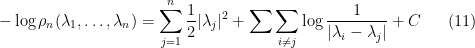
where  is a constant whose exact value is not of importance to us. From a mathematical physics perspective, one can interpret (11) as a Hamiltonian for particles at positions , subject to a confining harmonic potential (these are the
  terms) and a repulsive logarithmic potential between particles (these are the
  terms).
Our objective is now to find a distribution of that minimises this expression.
We know from previous notes that the should have magnitude  . Let us then heuristically make a mean field approximation, in that we approximate the discrete spectral measure
  by a continuous probability measure
  . (Secretly, we know from the semi-circular law that we should be able to take
  , but pretend that we do not know this fact yet.) Then we can heuristically approximate (11) as

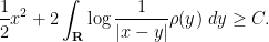
and so we expect the distribution  to minimise the functional

One can compute the Euler-Lagrange equations of this functional:
Exercise 6 Working formally, and assuming that is a probability measure that minimises (12), argue that

for some constant  and all
  in the support of . For all outside of the support, establish the inequality
There are various ways we can solve this equation for ; we sketch here a complex-analytic method. Differentiating in , we formally obtain

on the support of . But recall that if we let

be the Stieltjes transform of the probability measure , then we have

and
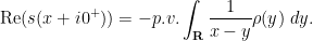
We conclude that

for all , which we rearrange as

This makes the function 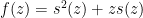 entire (it is analytic in the upper half-plane, obeys the symmetry
  , and has no jump across the real line). On the other hand, as
  as
as  ,
,  goes to
  at infinity. Applying Liouville’s theorem, we conclude that is constant, thus we have the familiar equation

which can then be solved to obtain the semi-circular law as in previous notes.
Remark 7 Recall from Notes 3b that Dyson Brownian motion can be used to derive the formula (1). One can then interpret the Dyson Brownian motion proof of the semi-circular law for GUE in Notes 4 as a rigorous formalisation of the above mean field approximation heuristic argument.
One can perform a similar heuristic analysis for the spectral measure  of a random gaussian matrix, giving a description of the limiting density:
Exercise 8 Using heuristic arguments similar to those above, argue that should be close to a continuous probability distribution  obeying the equation

on the support of , for some constant , with the inequality

outside of this support. Using the Newton potential  for the fundamental solution of the two-dimensional Laplacian
  , conclude (non-rigorously) that is equal to
  on its support.
Also argue that should be rotationally symmetric. Use (13) and Green’s formula to argue why the support of should be simply connected, and then conclude (again non-rigorously) the circular law

We will see more rigorous derivations of the circular law later in these notes, and also in subsequent notes.
— 4. Determinantal form of the GUE spectral distribution —
In a previous section, we showed (up to constants) that the density function for the eigenvalues of GUE was given by the formula (1).
As is well known, the Vandermonde determinant  that appears in (1) can be expressed up to sign as a determinant of an matrix, namely the matrix
  . Indeed, this determinant is clearly a polynomial of degree
  in which vanishes whenever two of the agree, and the claim then follows from the factor theorem (and inspecting a single coefficient of the Vandermonde determinant, e.g. the
  coefficient, to get the sign).
We can square the above fact (or more precisely, multiply the above matrix matrix by its adjoint) and conclude that  is the determinant of the matrix

More generally, if  are any sequence of polynomials, in which
  has degree
  , then we see from row operations that the determinant of

is a non-zero constant multiple of (with the constant depending on the leading coefficients of the  ), and so the determinant of

is a non-zero constant multiple of . Comparing this with (1), we obtain the formula

for some non-zero constant .
This formula is valid for any choice of polynomials of degree . But the formula is particularly useful when we set equal to the (normalised) Hermite polynomials, defined by applying the Gram-Schmidt process in  to the polynomials
  for
for  to yield
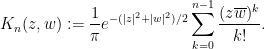
  . (Equivalently, the are the orthogonal polynomials associated to the measure
  .) In that case, the expression
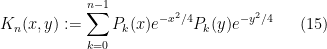
becomes the integral kernel of the orthogonal projection  operator in to the span of the , thus

for all  , and so
  is now a constant multiple of
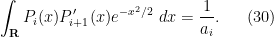
The reason for working with orthogonal polynomials is that we have the trace identity

and the reproducing formula

which reflects the identity  . These two formulae have an important consequence:
Lemma 9 (Determinantal integration formula) Let  be any symmetric rapidly decreasing function obeying (16), (17). Then for any
  , one has

Remark 10 This remarkable identity is part of the beautiful algebraic theory of determinantal processes, which I discuss further in this blog post.
Proof: We induct on  . When
  this is just (16). Now assume that
  and that the claim has already been proven for
  . We apply cofactor expansion to the bottom row of the determinant
  . This gives a principal term

plus a sum of additional terms, the  term of which is of the form

Using (16), the principal term (19) gives a contribution of  to (18). For each nonprincipal term (20), we use the multilinearity of the determinant to absorb the
  term into the
  column of the matrix. Using (17), we thus see that the contribution of (20) to (18) can be simplified as

which after row exchange, simplifies to  . The claim follows.
In particular, if we iterate the above lemma using the Fubini-Tonelli theorem, we see that

On the other hand, if we extend the probability density function symmetrically from the Weyl chamber  to all of
  , its integral is also . Since
  is clearly symmetric in the , we can thus compare constants and conclude the Gaudin-Mehta formula

More generally, if we define  to be the function

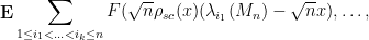
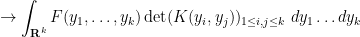
then the above formula shows that  is the -point correlation function for the spectrum, in the sense that


for any test function  supported in the region
  .
.
In particular, if we set  , we obtain the explicit formula
for the expected empirical spectral measure of . Equivalently after renormalising by  , we have

It is thus of interest to understand the kernel  better.
To do this, we begin by recalling that the functions were obtained from by the Gram-Schmidt process. In particular, each is orthogonal to the  for all
  . This implies that
  is orthogonal to for
  . On the other hand,
  is a polynomial of degree
  , so must lie in the span of for
  . Combining the two facts, we see that
  must be a linear combination of
  , with the
  coefficient being non-trivial. We rewrite this fact in the form

for some real numbers  (with
(with  ). Taking inner products with and
  we see that
and
and so

(with the convention  ).
).
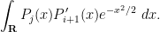
We will continue the computation of later. For now, we we pick two distinct real numbers  and consider the Wronskian-type expression

Using (24), (26), we can write this as

or in other words


We telescope this and obtain the Christoffel-Darboux formula for the kernel (15):

Sending  using L’Hopital’s rule, we obtain in particular that

Inserting this into (23), we see that if we want to understand the expected spectral measure of GUE, we should understand the asymptotic behaviour of  and the associated constants
  . For this, we need to exploit the specific properties of the gaussian weight
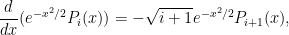
  . In particular, we have the identity
so upon integrating (25) by parts, we have

As  has degree at most
  , the first term vanishes by the orthonormal nature of the , thus
To compute this, let us denote the leading coefficient of as  . Then
  is equal to
  plus lower-order terms, and so we have

On the other hand, by inspecting the  coefficient of (24) we have

Combining the two formulae (and making the sign convention that the are always positive), we see that

and
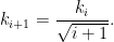
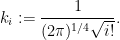
Meanwhile, a direct computation shows that  , and thus by induction
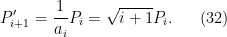
A similar method lets us compute the  . Indeed, taking inner products of (24) with
  and using orthonormality we have

which upon integrating by parts using (29) gives

As is of degree strictly less than , the integral vanishes by orthonormality, thus  . The identity (24) thus becomes Hermite recurrence relation

Another recurrence relation arises by considering the integral
On the one hand, as has degree at most , this integral vanishes if  by orthonormality. On the other hand, integrating by parts using (29), we can write the integral as

If  , then
  has degree less than , so the integral again vanishes. Thus the integral is non-vanishing only when
  . Using (30), we conclude that
We can combine (32) with (31) to obtain the formula
which together with the initial condition  gives the explicit representation

for the Hermite polynomials. Thus, for instance, at  one sees from Taylor expansion that

when is even, and

when is odd.
In principle, the formula (33), together with (28), gives us an explicit description of the kernel  (and thus of
  , by (23)). However, to understand the asymptotic behaviour as
  , we would have to understand the asymptotic behaviour of
  as , which is not immediately discernable by inspection. However, one can obtain such asymptotics by a variety of means. We give two such methods here: a method based on ODE analysis, and a complex-analytic method, based on the method of steepest descent.
We begin with the ODE method. Combining (31) with (32) we see that each polynomial  obeys the Hermite differential equation

If we look instead at the Hermite functions 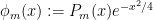 , we obtain the differential equation
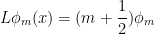
where  is the harmonic oscillator operator
Note that the self-adjointness of here is consistent with the orthogonal nature of the  .
.
Exercise 11 Use (15), (28), (33), (31), (32) to establish the identities

and thus by (23)
![\displaystyle = [\frac{1}{\sqrt{n}} \phi'_n(\sqrt{n} x)^2 + \sqrt{n} (1 - \frac{x^2}{4}) \phi_n(\sqrt{n} x)^2]\ dx.](https://s0.wp.com/latex.php?latex=%5Cdisplaystyle++%3D+%5B%5Cfrac%7B1%7D%7B%5Csqrt%7Bn%7D%7D+%5Cphi%27_n%28%5Csqrt%7Bn%7D+x%29%5E2+%2B+%5Csqrt%7Bn%7D+%281+-+%5Cfrac%7Bx%5E2%7D%7B4%7D%29+%5Cphi_n%28%5Csqrt%7Bn%7D+x%29%5E2%5D%5C+dx.&bg=ffffff&fg=000000&s=0&c=20201002)
It is thus natural to look at the rescaled functions
which are orthonormal in and solve the equation

where  is the semiclassical harmonic oscillator operator

thus

![\displaystyle = [\frac{1}{n^2} \tilde \phi'_n(x)^2 + (1 - \frac{x^2}{4}) \tilde \phi_n(x)^2]\ dx. \ \ \ \ \ (36)](https://s0.wp.com/latex.php?latex=%5Cdisplaystyle++%3D+%5B%5Cfrac%7B1%7D%7Bn%5E2%7D+%5Ctilde+%5Cphi%27_n%28x%29%5E2+%2B+%281+-+%5Cfrac%7Bx%5E2%7D%7B4%7D%29+%5Ctilde+%5Cphi_n%28x%29%5E2%5D%5C+dx.+%5C+%5C+%5C+%5C+%5C+%2836%29&bg=ffffff&fg=000000&s=0&c=20201002)
The projection is then the spectral projection operator of  to
to ![{[0,1]}](https://s0.wp.com/latex.php?latex=%7B%5B0%2C1%5D%7D&bg=ffffff&fg=000000&s=0&c=20201002) . According to semi-classical analysis, with
. According to semi-classical analysis, with  being interpreted as analogous to Planck’s constant, the operator has symbol
  , where
  is the momentum operator, so the projection is a projection to the region
  of phase space, or equivalently to the region
  . In the semi-classical limit
  , we thus expect the diagonal of the normalised projection
  to be proportional to the projection of this region to the variable, i.e. proportional to
  . We are thus led to the semi-circular law via semi-classical analysis.
It is possible to make the above argument rigorous, but this would require developing the theory of microlocal analysis, which would be overkill given that we are just dealing with an ODE rather than a PDE here (and an extremely classical ODE at that). We instead use a more basic semiclassical approximation, the WKB approximation, which we will make rigorous using the classical method of variation of parameters (one could also proceed using the closely related Prüfer transformation, which we will not detail here). We study the eigenfunction equation

where we think of  as being small, and as being close to . We rewrite this as
where  , where we will only work in the “classical” region
  (so
(so  ) for now.
Recall that the general solution to the constant coefficient ODE  is given by
  . Inspired by this, we make the ansatz

where  is the antiderivative of . Differentiating this, we have


Because we are representing a single function  by two functions
  , we have the freedom to place an additional constraint on
  . Following the usual variation of parameters strategy, we will use this freedom to eliminate the last two terms in the expansion of , thus

We can now differentiate again and obtain


Comparing this with (37) we see that

Combining this with (38), we obtain equations of motion for  and
and  :
:
We can simplify this using the integrating factor substitution

to obtain

The point of doing all these transformations is that the role of the parameter no longer manifests itself through amplitude factors, and instead only is present in a phase factor. In particular, we have
on any compact interval  in the interior of the classical region (where we allow implied constants to depend on ), which by Gronwall’s inequality gives the bounds

on this interval . We can then insert these bounds into (39), (40) again and integrate by parts (taking advantage of the non-stationary nature of  ) to obtain the improved bounds

on this interval. (More precise asymptotic expansions can be obtained by iterating this procedure, but we will not need them here.) This is already enough to get the asymptotics that we need:
Exercise 12 Use (36) to Show that on any compact interval in  , the density of is given by

where  are as above with
  and
and  . Combining this with (41), (34), (35), and Stirling’s formula, conclude that converges in the vague topology to the semicircular law
  . (Note that once one gets convergence inside , the convergence outside of
 ![{[-2,2]}](https://s0.wp.com/latex.php?latex=%7B%5B-2%2C2%5D%7D&bg=ffffff&fg=000000&s=0&c=20201002) can be obtained for free since
can be obtained for free since  and are both probability measures.
We now sketch out the approach using the method of steepest descent. The starting point is the Fourier inversion formula

which upon repeated differentiation gives

and thus by (33)

and thus

where

where we use a suitable branch of the complex logarithm to handle the case of negative  .
.
The idea of the principle of steepest descent is to shift the contour of integration to where the real part of  is as small as possible. For this, it turns out that the stationary points of play a crucial role. A brief calculation using the quadratic formula shows that there are two such stationary points, at
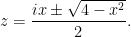
When  , is purely imaginary at these stationary points, while for
  the real part of is negative at both points. One then draws a contour through these two stationary points in such a way that near each such point, the imaginary part of is kept fixed, which keeps oscillation to a minimum and allows the real part to decay as steeply as possible (which explains the name of the method). After a certain tedious amount of computation, one obtains the same type of asymptotics for
  that were obtained by the ODE method when (and exponentially decaying estimates for
  ).
).
Exercise 13 Let  ,
,  be functions which are analytic near a complex number
  , with
  and
and  . Let be a small number, and let
  be the line segment
  , where
  is a complex phase such that
  is a negative real. Show that for sufficiently small, one has

as  . This is the basic estimate behind the method of steepest descent; readers who are also familiar with the method of stationary phase may see a close parallel.
Remark 14 The method of steepest descent requires an explicit representation of the orthogonal polynomials as contour integrals, and as such is largely restricted to the classical orthogonal polynomials (such as the Hermite polynomials). However, there is a non-linear generalisation of the method of steepest descent developed by Deift and Zhou, in which one solves a matrix Riemann-Hilbert problem rather than a contour integral; see this book by Deift for details. Using these sorts of tools, one can generalise much of the above theory to the spectral distribution of -conjugation-invariant discussed in Remark 2, with the theory of Hermite polynomials being replaced by the more general theory of orthogonal polynomials; this is discussed in the above book of Deift, as well as the more recent book of Deift and Gioev.
The computations performed above for the diagonal kernel can be summarised by the asymptotic

whenever  is fixed and , and
 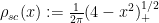 is the semi-circular law distribution. It is reasonably straightforward to generalise these asymptotics to the off-diagonal case as well, obtaining the more general result

for fixed  and
and  , where
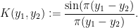
  is the Dyson sine kernel
In the language of semi-classical analysis, what is going on here is that the rescaling in the left-hand side of (42) is transforming the phase space region to the region  in the limit , and the projection to the latter region is given by the Dyson sine kernel. A formal proof of (42) can be given by using either the ODE method or the steepest descent method to obtain asymptotics for Hermite polynomials, and thence (via the Christoffel-Darboux formula) to asymptotics for ; we do not give the details here, but see for instance the recent book of Anderson, Guionnet, and Zeitouni.
From (42) and (21), (22) we obtain the asymptotic formula

for the local statistics of eigenvalues. By means of further algebraic manipulations (using the general theory of determinantal processes), this allows one to control such quantities as the distribution of eigenvalue gaps near  , normalised at the scale
  , which is the average size of these gaps as predicted by the semicircular law. For instance, for any
  , one can show (basically by the above formulae combined with the inclusion-exclusion principle) that the proportion of eigenvalues with normalised gap
  less than
  converges as to
 ![{\int_0^{s_0} \frac{d^2}{ds^2} \det(1-K)_{L^2[0,s]}\ ds}](https://s0.wp.com/latex.php?latex=%7B%5Cint_0%5E%7Bs_0%7D+%5Cfrac%7Bd%5E2%7D%7Bds%5E2%7D+%5Cdet%281-K%29_%7BL%5E2%5B0%2Cs%5D%7D%5C+ds%7D&bg=ffffff&fg=000000&s=0&c=20201002) , where
, where ![{t_c \in [-2,2]}](https://s0.wp.com/latex.php?latex=%7Bt_c+%5Cin+%5B-2%2C2%5D%7D&bg=ffffff&fg=000000&s=0&c=20201002) is defined by the formula
is defined by the formula  , and is the integral operator with kernel
  (this operator can be verified to be trace class, so the determinant can be defined in a Fredholm sense). See for instance this book of Mehta (and my blog post on determinantal processes describe a finitary version of the inclusion-exclusion argument used to obtain such a result).
Remark 15 One can also analyse the distribution of the eigenvalues at the edge of the spectrum, i.e. close to  . This ultimately hinges on understanding the behaviour of the projection near the corners
  of the phase space region
  , or of the Hermite polynomials
  for close to . For instance, by using steepest descent methods, one can show that

as for any fixed , where  is the Airy function
This asymptotic and the Christoffel-Darboux formula then gives the asymptotic

for any fixed , where  is the Airy kernel

(Aside: Semiclassical heuristics suggest that the rescaled kernel (43) should correspond to projection to the parabolic region of phase space  , but I do not know of a connection between this region and the Airy kernel; I am not sure whether semiclassical heuristics are in fact valid at this scaling regime. On the other hand, these heuristics do explain the emergence of the length scale
  that emerges in (43), as this is the smallest scale at the edge which occupies a region in
  consistent with the Heisenberg uncertainty principle.) This then gives an asymptotic description of the largest eigenvalues of a GUE matrix, which cluster in the region
  . For instance, one can use the above asymptotics to show that the largest eigenvalue
  of a GUE matrix obeys the Tracy-Widom law
![\displaystyle \mathop{\bf P}( \frac{\lambda_1 - 2\sqrt{n}}{n^{1/6}} < t ) \rightarrow \det(1 - A)_{L^2[0,t]}](https://s0.wp.com/latex.php?latex=%5Cdisplaystyle++%5Cmathop%7B%5Cbf+P%7D%28+%5Cfrac%7B%5Clambda_1+-+2%5Csqrt%7Bn%7D%7D%7Bn%5E%7B1%2F6%7D%7D+%3C+t+%29+%5Crightarrow+%5Cdet%281+-+A%29_%7BL%5E2%5B0%2Ct%5D%7D&bg=ffffff&fg=000000&s=0&c=20201002)
for any fixed , where is the integral operator with kernel . See for instance the recent book of Anderson, Guionnet, and Zeitouni.
— 5. Determinantal form of the gaussian matrix distribution —
One can perform an analogous analysis of the joint distribution function (10) of gaussian random matrices. Indeed, given any family  of polynomials, with each of degree , much the same arguments as before show that (10) is equal to a constant multiple of
One can then select  to be orthonormal in
  . Actually in this case, the polynomials are very simple, being given explicitly by the formula

Exercise 16 Verify that the are indeed orthonormal, and then conclude that (10) is equal to  , where
Conclude further that the  -point correlation functions
  are given as

Exercise 17 Show that as , one has
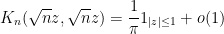
and deduce that the expected spectral measure  converges vaguely to the circular measure
 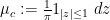 ; this is a special case of the circular law.
Exercise 18 For any  and
and  , show that

as . This formula (in principle, at least) describes the asymptotic local -point correlation functions of the spectrum of gaussian matrices.
Remark 19 One can use the above formulae as the starting point for many other computations on the spectrum of random gaussian matrices; to give just one example, one can show that expected number of eigenvalues which are real is of the order of (see this paper of Edelman for more precise results of this nature). It remains a challenge to extend these results to more general ensembles than the gaussian ensemble.


24 comments
Comments feed for this article
24 February, 2010 at 11:48 am
Anonymous
There’s a minor typo (“frac” should be “\frac”) in the statement of Exercise 9.
[Corrected, thanks – T.]
26 February, 2010 at 6:49 pm
Anonymous
Dear Prof. Tao,
Thank you for the great post.
Which course are you going to teach next semester? If you give a hint, we can start to read related materials. your lecture notes are terrific but requires strong background.
Thanks
5 March, 2010 at 1:47 pm
254A, Notes 7: The least singular value « What’s new
[…] of a gaussian random matrix can be computed explicitly by techniques similar to those employed in Notes 6. In particular, if is a real gaussian matrix (with all entries iid with distribution ), it was […]
9 August, 2010 at 10:31 am
Anonymous
In deriving the pdf for GUE, “We can thus use the inverse function theorem in this local region of parameter space and make the ansatz ….”
How is this true? Is there any reference to detailing this step?
9 August, 2010 at 12:46 pm
Terence Tao
As stated immediately after that quote, one computes the Jacobian of at
at  (and
(and  equal to a diagonal unitary) and verifies that it is non-zero. This already gives the desired parameterisation in the
  neighbourhood of any diagonal unitary
  , from the inverse function theorem (it may be convenient here to scale out the
  and look at the map
  instead). Since we already know
  lies within
  of a diagonal unitary, the claim follows.
23 October, 2010 at 12:57 pm
The Dyson and Airy kernels of GUE via semiclassical analysis « What’s new
[…] standard computation (given for instance in these lecture notes of mine) gives the Ginebre […]
4 December, 2010 at 10:44 pm
Anonymous
Dear Prof. Tao,
I don’t quite understand the argument after equation (20). You said you want to absorb K_n(x_l,x_{k+1}) into the l-th column. But isn’t the l-th column omitted in the matrix that follows? Maybe you meant the k+1th column? But I couldn’t figure out how to make it work.
[Corrected, thanks. The strategy is to get to the point where one can use the identity .]
.]
5 December, 2010 at 11:32 am
Anonymous
Ah I see. You are integrating partially first. Thanks!
2 November, 2011 at 1:30 pm
Smolin (2011) | Research Notebook
[…] is a real valued random matrix from the GOE ensemble whose eigenvalues for subscribe to Dyson Brownian […]
15 June, 2012 at 5:31 am
vishwajeet singh
Dear Dr Tao,
I have just started my venture into Random matrix. What puzzles me is that all the Gaussian ensembles assume zero mean entries. How does the entire formulation change when the entries do not have zero mean? i.e the entries are Normal(\mu,\sigma). How does the distribution of the eigenvalues change ??
Thanks.
12 November, 2012 at 7:59 am
A direct proof of the stationarity of the Dyson sine process under Dyson Brownian motion « What’s new
[…] where are the (normalised) Hermite polynomials; see this previous blog post for details. […]
17 March, 2013 at 8:26 pm
Ilya Razenshteyn
My feeling that is (43) the normalization is wrong. There should be .
.
[Corrected, thanks – T.]
5 January, 2014 at 3:09 am
Anonymous
In Section 2, doesn’t conjugation by a permutation matrix make T lose its upper diagonal structure?
5 January, 2014 at 10:16 am
Terence Tao
Gah, you’re right. Fortunately, the permutation symmetry for T is not actually needed in the argument, provided that one augments the given data (i.e. the matrix G to be factorised) by also attaching a (randomly chosen) enumeration of the eigenvalues of G, and demanding that T has the diagonal entries
  in that order. While T indeed does not have permutation symmetry, the data (the pair consisting of
  and the enumeration
  ) retains the permutation symmetry, which is what is actually used in the argument. I’ve rewritten the text to reflect this.
2 March, 2015 at 1:59 pm
Chansoo Lee
Dear Professor Tao,
Does the fact that you used a heuristic mean field approximation imply that in general, you can’t find the actual eigenvalues that maximize the pdf for n > 4?
Thanks
2 March, 2015 at 8:36 pm
Terence Tao
The points that maximise the pdf are known as Fekete points; asymptotics for these points are known (by using a more rigorous version of the mean field approximation), but I doubt that there is any closed form for them.
29 June, 2016 at 3:10 pm
Jhon Manugal
I know it’s a cheap trick, but you should definitely use raising and lowering operators since you are dealing with Hermite polynomials. And there’s probably an representation or
  in there but don’t take my word for it. I appreciate you doing WKB approximation in a rigorous way but I had trouble recognizing it compared to what the physicists actually write. So Ratner theorem, WKB approximation and everything else is the same.
5 January, 2017 at 11:27 am
Ramis Movassagh
Hi Terry, A minor typo perhaps.
On the 5th line, in the paragraph above Eq. 2 starting with ” Let D be…”, M should probably be M_n.
[Corrected, thanks -T.]
8 January, 2017 at 9:54 am
Ramis Movassagh
Hi Terry,
I very much like this post as always.
Minor typos perhaps:
The first paragraph below Eq. 11 the I think instead of 1/|\lambda_i – \lambda_j|, it should say \log 1/|\lambda_i – \lambda_j|.
Also three lines below “\lambda_i should be have…” to “\lambda_i should have…”
[Corrected, thanks – T.]
8 April, 2019 at 8:07 am
Anonymous
Dear professor Tao
Right after making the ansatz {U=\exp(\epsilon S)R} you say
As {U} is distributed using Haar measure on {U(n)}, {S} is (locally) distributed using {\epsilon^{n^2-n}} times a constant multiple of Lebesgue measure on the space {W} of skew-adjoint matrices with zero diagonal, which has dimension {n^2-n}.
Is there any refference to this step in details? Do i need to use the Baker–Campbell–Hausdorff formula?
8 April, 2019 at 11:10 am
Terence Tao
Oops, there was a factor of missing in front of
  . One can indeed proceed using BCH: the fact that Haar measure is invariant under rotations of the form
  for some skew-adjoint
  with zero diagonal means that the distribution of S is invariant under a transformation which looks like translation by
  plus errors of size
  (and whose derivatives also have size o(1)), so after taking Jacobians we see that the density of this distribution is constant up to factors of
  .
.
10 May, 2019 at 8:37 am
The alternative hypothesis for unitary matrices | What's new
[…] the the Vandermonde determinant; see for instance this previous blog post for the derivation of a very similar formula for the GUE distribution, which can be adapted to CUE […]
3 January, 2021 at 12:50 am
tpfly
Dear Professor Tao,
In Exercise 4 should there be a factor of 2 before the logarithmic potential? Otherwise taking the Laplacian we would get $\rho(z)=2/\pi$ on its support.
[Corrected, thanks – T.]
18 January, 2021 at 1:56 am
tpfly
Dear Professor Tao,
The HTML code has been broken since last modification, and some latex formula do not parse.
I think there are still some more mistakes in this post and in the corresponding chapter of “topics in RMT”:
1): Using (34), I found (35) should be
when n is odd. Comparing with (35), the sign is different (the power of -1 should be (n-1)/2).
2) The rescaled functions should be defined as
  which are orthonormal. The scale
  outside of the functions do not make them orthonormal.
 should be
  instead of
  .
. should be
  .
. (in the sketch of steepest descent), the factor
  is missing.
Then the following 3), 4), 5) are related to this.
3) In the book, the harmonic oscillator operator on
4) In eq.(36), the coefficient of
5) In the integral formula of
6) In Exercise 12, the density of should be
[Corrected, thanks – T.]