In a recent post I discussed how the Riemann zeta function  can be locally approximated by a polynomial, in the sense that for randomly chosen
 ![{t \in [T,2T]}](https://s0.wp.com/latex.php?latex=%7Bt+%5Cin+%5BT%2C2T%5D%7D&bg=ffffff&fg=000000&s=0&c=20201002) one has an approximation
one has an approximation

where  grows slowly with
  , and
, and  is a polynomial of degree . Assuming the Riemann hypothesis (as we will throughout this post), the zeroes of should all lie on the unit circle, and one should then be able to write as a scalar multiple of the characteristic polynomial of (the inverse of) a unitary matrix
  , which we normalise as

Here  is some quantity depending on
  . We view
  as a random element of
  ; in the limit
  , the GUE hypothesis is equivalent to becoming equidistributed with respect to Haar measure on (also known as the Circular Unitary Ensemble, CUE; it is to the unit circle what the Gaussian Unitary Ensemble (GUE) is on the real line). One can also view as analogous to the “geometric Frobenius” operator in the function field setting, though unfortunately it is difficult at present to make this analogy any more precise (due, among other things, to the lack of a sufficiently satisfactory theory of the “field of one element“).
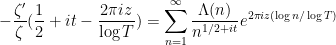
Taking logarithmic derivatives of (2), we have

and hence on taking logarithmic derivatives of (1) in the  variable we (heuristically) have

Morally speaking, we have
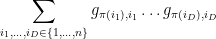
so on comparing coefficients we expect to interpret the moments  of as a finite Dirichlet series:
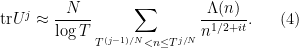
To understand the distribution of in the unitary group , it suffices to understand the distribution of the moments

where  denotes averaging over , and
  . The GUE hypothesis asserts that in the limit , these moments converge to their CUE counterparts

where is now drawn uniformly in  with respect to the CUE ensemble, and
  denotes expectation with respect to that measure.
The moment (6) vanishes unless one has the homogeneity condition

This follows from the fact that for any phase  ,
,  has the same distribution as , where we use the number theory notation
  .
.
In the case when the degree  is low, we can use representation theory to establish the following simple formula for the moment (6), as evaluated by Diaconis and Shahshahani:
Proposition 1 (Low moments in CUE model) If

then the moment (6) vanishes unless  for all
  , in which case it is equal to

Another way of viewing this proposition is that for distributed according to CUE, the random variables are distributed like independent complex random variables of mean zero and variance , as long as one only considers moments obeying (8). This identity definitely breaks down for larger values of  , so one only obtains central limit theorems in certain limiting regimes, notably when one only considers a fixed number of ‘s and lets go to infinity. (The paper of Diaconis and Shahshahani writes
  in place of , but I believe this to be a typo.)
Proof: Let  be the left-hand side of (8). We may assume that (7) holds since we are done otherwise, hence

Our starting point is Schur-Weyl duality. Namely, we consider the  -dimensional complex vector space

This space has an action of the product group  : the symmetric group
  acts by permutation on the tensor factors, while the general linear group
  acts diagonally on the
  factors, and the two actions commute with each other. Schur-Weyl duality gives a decomposition
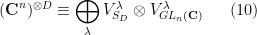
where  ranges over Young tableaux of size with at most
  rows,
rows,  is the -irreducible unitary representation corresponding to (which can be constructed for instance using Specht modules), and
  is the -irreducible polynomial representation corresponding with highest weight .
Let  be a permutation consisting of cycles of length (this is uniquely determined up to conjugation), and let
  . The pair
  then acts on
  , with the action on basis elements
  given by
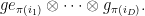
The trace of this action can then be computed as
where  is the
  matrix coefficient of
  . Breaking up into cycles and summing, this is just

But we can also compute this trace using the Schur-Weyl decomposition (10), yielding the identity

where  is the character on associated to , and
  is the character on associated to . As is well known,
  is just the Schur polynomial of weight applied to the (algebraic, generalised) eigenvalues of . We can specialise to unitary matrices to conclude that

and similarly

where  consists of
  cycles of length for each
  . On the other hand, the characters
  are an orthonormal system on
  with the CUE measure. Thus we can write the expectation (6) as

Now recall that ranges over all the Young tableaux of size with at most rows. But by (8) we have  , and so the condition of having rows is redundant. Hence now ranges over all Young tableaux of size , which as is well known enumerates all the irreducible representations of . One can then use the standard orthogonality properties of characters to show that the sum (12) vanishes if
  ,
,  are not conjugate, and is equal to
  divided by the size of the conjugacy class of (or equivalently, by the size of the centraliser of ) otherwise. But the latter expression is easily computed to be
  , giving the claim.
Example 2 We illustrate the identity (11) when  ,
,  . The Schur polynomials are given as


where  are the (generalised) eigenvalues of , and the formula (11) in this case becomes


The functions  are orthonormal on , so the three functions
  are also, and their
  norms are
  ,
,  , and
, and  respectively, reflecting the size in
  of the centralisers of the permutations
  ,
,  , and
, and  respectively. If is instead set to say
  , then the
  terms now disappear (the Young tableau here has too many rows), and the three quantities here now have some non-trivial covariance.
Example 3 Consider the moment  . For
. For  , the above proposition shows us that this moment is equal to . What happens for
  ? The formula (12) computes this moment as

where is a cycle of length in  , and ranges over all Young tableaux with size and at most rows. The Murnaghan-Nakayama rule tells us that
  vanishes unless is a hook (all but one of the non-zero rows consisting of just a single box; this also can be interpreted as an exterior power representation on the space
  of vectors in
  whose coordinates sum to zero), in which case it is equal to
  (depending on the parity of the number of non-zero rows). As such we see that this moment is equal to . Thus in general we have

Now we discuss what is known for the analogous moments (5). Here we shall be rather non-rigorous, in particular ignoring an annoying “Archimedean” issue that the product of the ranges  and
and  is not quite the range
  but instead leaks into the adjacent range
  . This issue can be addressed by working in a “weak" sense in which parameters such as
  are averaged over fairly long scales, or by passing to a function field analogue of these questions, but we shall simply ignore the issue completely and work at a heuristic level only. For similar reasons we will ignore some technical issues arising from the sharp cutoff of to the range
 ![{[T,2T]}](https://s0.wp.com/latex.php?latex=%7B%5BT%2C2T%5D%7D&bg=ffffff&fg=000000&s=0&c=20201002) (it would be slightly better technically to use a smooth cutoff).
(it would be slightly better technically to use a smooth cutoff).
One can morally expand out (5) using (4) as


where  ,
,  , and the integers
  are in the ranges

for and  , and
, and

for and  . Morally, the expectation here is negligible unless

in which case the expecation is oscillates with magnitude one. In particular, if (7) fails (with some room to spare) then the moment (5) should be negligible, which is consistent with the analogous behaviour for the moments (6). Now suppose that (8) holds (with some room to spare). Then  is significantly less than , so the
  multiplicative error in (15) becomes an additive error of
  . On the other hand, because of the fundamental integrality gap – that the integers are always separated from each other by a distance of at least
  – this forces the integers
  , to in fact be equal:

The von Mangoldt factors  effectively restrict
  to be prime (the effect of prime powers is negligible). By the fundamental theorem of arithmetic, the constraint (16) then forces
  , and
, and  to be a permutation of
  , which then forces
  for all ._ For a given , the number of possible is then
  , and the expectation in (14) is equal to . Thus this expectation is morally
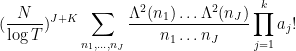
and using Mertens’ theorem this soon simplifies asymptotically to the same quantity in Proposition 1. Thus we see that (morally at least) the moments (5) associated to the zeta function asymptotically match the moments (6) coming from the CUE model in the low degree case (8), thus lending support to the GUE hypothesis. (These observations are basically due to Rudnick and Sarnak, with the degree case of pair correlations due to Montgomery, and the degree case due to Hejhal.)
With some rare exceptions (such as those estimates coming from “Kloostermania”), the moment estimates of Rudnick and Sarnak basically represent the state of the art for what is known for the moments (5). For instance, Montgomery’s pair correlation conjecture, in our language, is basically the analogue of (13) for  , thus

for all  . Montgomery showed this for (essentially) the range (as remarked above, this is a special case of the Rudnick-Sarnak result), but no further cases of this conjecture are known.
These estimates can be used to give some non-trivial information on the largest and smallest spacings between zeroes of the zeta function, which in our notation corresponds to spacing between eigenvalues of . One such method used today for this is due to Montgomery and Odlyzko and was greatly simplified by Conrey, Ghosh, and Gonek. The basic idea, translated to our random matrix notation, is as follows. Suppose  is some random polynomial depending on of degree at most . Let denote the eigenvalues of , and let
  be a parameter. Observe from the pigeonhole principle that if the quantity

exceeds the quantity

then the arcs  cannot all be disjoint, and hence there exists a pair of eigenvalues making an angle of less than
  (
( times the mean angle separation). Similarly, if the quantity (18) falls below that of (19), then these arcs cannot cover the unit circle, and hence there exists a pair of eigenvalues making an angle of greater than times the mean angle separation. By judiciously choosing the coefficients of
  as functions of the moments
  , one can ensure that both quantities (18), (19) can be computed by the Rudnick-Sarnak estimates (or estimates of equivalent strength); indeed, from the residue theorem one can write (18) as

for sufficiently small  , and this can be computed (in principle, at least) using (3) if the coefficients of are in an appropriate form. Using this sort of technology (translated back to the Riemann zeta function setting), one can show that gaps between consecutive zeroes of zeta are less than
  times the mean spacing and greater than times the mean spacing infinitely often for certain
  ; the current records are
  (due to Goldston and Turnage-Butterbaugh) and
  (due to Bui and Milinovich, who input some additional estimates beyond the Rudnick-Sarnak set, namely the twisted fourth moment estimates of Bettin, Bui, Li, and Radziwill, and using a technique based on Hall’s method rather than the Montgomery-Odlyzko method).
It would be of great interest if one could push the upper bound for the smallest gap below  . The reason for this is that this would then exclude the Alternative Hypothesis that the spacing between zeroes are asymptotically always (or almost always) a non-zero half-integer multiple of the mean spacing, or in our language that the gaps between the phases
  of the eigenvalues
  of are nasymptotically always non-zero integer multiples of
  . The significance of this hypothesis is that it is implied by the existence of a Siegel zero (of conductor a small power of ); see this paper of Conrey and Iwaniec. (In our language, what is going on is that if there is a Siegel zero in which
  is very close to zero, then
  behaves like the Kronecker delta, and hence (by the Riemann-Siegel formula) the combined
  -function
  will have a polynomial approximation which in our language looks like a scalar multiple of
  , where
  and is a phase. The zeroes of this approximation lie on a coset of the
  roots of unity; the polynomial
  is a factor of this approximation and hence will also lie in this coset, implying in particular that all eigenvalue spacings are multiples of
  . Taking
  then gives the claim.)
Unfortunately, the known methods do not seem to break this barrier without some significant new input; already the original paper of Montgomery and Odlyzko observed this limitation for their particular technique (and in fact fall very slightly short, as observed in unpublished work of Goldston and of Milinovich). In this post I would like to record another way to see this, by providing an “alternative” probability distribution to the CUE distribution (which one might dub the Alternative Circular Unitary Ensemble (ACUE) which is indistinguishable in low moments in the sense that the expectation  for this model also obeys Proposition 1, but for which the phase spacings are always a multiple of . This shows that if one is to rule out the Alternative Hypothesis (and thus in particular rule out Siegel zeroes), one needs to input some additional moment information beyond Proposition 1. It would be interesting to see if any of the other known moment estimates that go beyond this proposition are consistent with this alternative distribution. (UPDATE: it looks like they are, see Remark 7 below.)
To describe this alternative distribution, let us first recall the Weyl description of the CUE measure on the unitary group in terms of the distribution of the phases  of the eigenvalues, randomly permuted in any order. This distribution is given by the probability measure
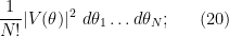
where

is the Vandermonde determinant; see for instance this previous blog post for the derivation of a very similar formula for the GUE distribution, which can be adapted to CUE without much difficulty. To see that this is a probability measure, first observe the Vandermonde determinant identity

where  ,
,  denotes the dot product, and
  is the “long word”, which implies that (20) is a trigonometric series with constant term ; it is also clearly non-negative, so it is a probability measure. One can thus generate a random CUE matrix by first drawing
  using the probability measure (20), and then generating to be a random unitary matrix with eigenvalues
  .
.
For the alternative distribution, we first draw  on the discrete torus
  (thus each
  is a
is a  root of unity) with probability density function

shift by a phase  drawn uniformly at random, and then select to be a random unitary matrix with eigenvalues
  . Let us first verify that (21) is a probability density function. Clearly it is non-negative. It is the linear combination of exponentials of the form
  for
for  . The diagonal contribution
  gives the constant function
  , which has total mass one. All of the other exponentials have a frequency
  that is not a multiple of
  , and hence will have mean zero on . The claim follows.
From construction it is clear that the matrix drawn from this alternative distribution will have all eigenvalue phase spacings be a non-zero multiple of . Now we verify that the alternative distribution also obeys Proposition 1. The alternative distribution remains invariant under rotation by phases, so the claim is again clear when (8) fails. Inspecting the proof of that proposition, we see that it suffices to show that the Schur polynomials with of size at most and of equal size remain orthonormal with respect to the alternative measure. That is to say,

when  have size equal to each other and at most . In this case the phase
  in the definition of is irrelevant. In terms of eigenvalue measures, we are then reduced to showing that

By Fourier decomposition, it then suffices to show that the trigonometric polynomial  does not contain any components of the form
  for some non-zero lattice vector
  . But we have already observed that
  is a linear combination of plane waves of the form for . Also, as is well known,
  is a linear combination of plane waves
  where
where  is majorised by , and similarly
  is a linear combination of plane waves
  where
where  is majorised by
  . So the product is a linear combination of plane waves of the form
  . But every coefficient of the vector
  lies between
  and
and  , and so cannot be of the form
  for any non-zero lattice vector
  , giving the claim.
Example 4 If  , then the distribution (21) assigns a probability of
  to any pair
  that is a permuted rotation of
  , and a probability of
  to any pair that is a permuted rotation of
  . Thus, a matrix drawn from the alternative distribution will be conjugate to a phase rotation of
  with probability , and to
  with probability .
A similar computation when  gives conjugate to a phase rotation of
  with probability
  , to a phase rotation of
  or its adjoint with probability of
  each, and a phase rotation of
  with probability
  .
.
Remark 5 For large it does not seem that this specific alternative distribution is the only distribution consistent with Proposition 1 and which has all phase spacings a non-zero multiple of ; in particular, it may not be the only distribution consistent with a Siegel zero. Still, it is a very explicit distribution that might serve as a test case for the limitations of various arguments for controlling quantities such as the largest or smallest spacing between zeroes of zeta. The ACUE is in some sense the distribution that maximally resembles CUE (in the sense that it has the greatest number of Fourier coefficients agreeing) while still also being consistent with the Alternative Hypothesis, and so should be the most difficult enemy to eliminate if one wishes to disprove that hypothesis.
In some cases, even just a tiny improvement in known results would be able to exclude the alternative hypothesis. For instance, if the alternative hypothesis held, then  is periodic in with period , so from Proposition 1 for the alternative distribution one has

which differs from (13) for any  . (This fact was implicitly observed recently by Baluyot, in the original context of the zeta function.) Thus a verification of the pair correlation conjecture (17) for even a single with would rule out the alternative hypothesis. Unfortunately, such a verification appears to be on comparable difficulty with (an averaged version of) the Hardy-Littlewood conjecture, with power saving error term. (This is consistent with the fact that Siegel zeroes can cause distortions in the Hardy-Littlewood conjecture, as (implicitly) discussed in this previous blog post.)
Remark 6 One can view the CUE as normalised Lebesgue measure on (viewed as a smooth submanifold of  ). One can similarly view ACUE as normalised Lebesgue measure on the (disconnected) smooth submanifold of consisting of those unitary matrices whose phase spacings are non-zero integer multiples of ; informally, ACUE is CUE restricted to this lower dimensional submanifold. As is well known, the phases of CUE eigenvalues form a determinantal point process with kernel
  (or one can equivalently take
  ; in a similar spirit, the phases of ACUE eigenvalues, once they are rotated to be roots of unity, become a discrete determinantal point process on those roots of unity with exactly the same kernel (except for a normalising factor of
  ). In particular, the -point correlation functions of ACUE (after this rotation) are precisely the restriction of the -point correlation functions of CUE after normalisation, that is to say they are proportional to
  .
.
Remark 7 One family of estimates that go beyond the Rudnick-Sarnak family of estimates are twisted moment estimates for the zeta function, such as ones that give asymptotics for

for some small even exponent  (almost always or
  ) and some short Dirichlet polynomial
  ; see for instance this paper of Bettin, Bui, Li, and Radziwill for some examples of such estimates. The analogous unitary matrix average would be something like

where is now some random medium degree polynomial that depends on the unitary matrix associated to (and in applications will typically also contain some negative power of  to cancel the corresponding powers of in
  ). Unfortunately such averages generally are unable to distinguish the CUE from the ACUE. For instance, if all the coefficients of involve products of traces
  of total order less than
  , then in terms of the eigenvalue phases ,
  is a linear combination of plane waves
  where the frequencies
  have coefficients of magnitude less than . On the other hand, as each coefficient of is an elementary symmetric function of the eigenvalues,
  is a linear combination of plane waves where the frequencies have coefficients of magnitude at most . Thus
  is a linear combination of plane waves where the frequencies have coefficients of magnitude less than , and thus is orthogonal to the difference between the CUE and ACUE measures on the phase torus
  by the previous arguments. In other words, has the same expectation with respect to ACUE as it does with respect to CUE. Thus one can only start distinguishing CUE from ACUE if the mollifier has degree close to or exceeding , which corresponds to Dirichlet polynomials of length close to or exceeding , which is far beyond current technology for such moment estimates.
Remark 8 The GUE hypothesis for the zeta function asserts that the average

is equal to

for any  and any test function
  , where
  is the Dyson sine kernel and
  are the ordinates of zeroes of the zeta function. This corresponds to the CUE distribution for . The ACUE distribution then corresponds to an “alternative gaussian unitary ensemble (AGUE)” hypothesis, in which the average (22) is instead predicted to equal a Riemann sum version of the integral (23):

This is a stronger version of the alternative hypothesis that the spacing between adjacent zeroes is almost always approximately a half-integer multiple of the mean spacing. I do not know of any known moment estimates for Dirichlet series that is able to eliminate this AGUE hypothesis (even assuming GRH). (UPDATE: These facts have also been independently observed in forthcoming work of Lagarias and Rodgers.)


30 comments
Comments feed for this article
9 May, 2019 at 2:27 am
Raphael
I like that N grow slowly with N in the introduction ;-)
[Corrected, thanks – T.]
9 May, 2019 at 4:40 am
Anonymous
It should be added that the bounds for consecutive nontrivial zeta zeros are only in the “infinitely often” sense.
[Corrected, thanks – T.]
9 May, 2019 at 5:33 am
Joseph
Is it expected that there is a similar limitation for larger gaps, i.e. one can construct a random matrix model such that the Schur functions of size at most remain orthonormal, and the maximal gap is bounded by
  for some constant
  ?
?
9 May, 2019 at 7:36 am
Terence Tao
I don’t know of such a limitation, and indeed there seems to be considerably more scope to improve the bounds on than on
  . For instance, the current best bound 0.515396 for
  only improves very slightly on the previous record 0.515398 of Feng and Xu, and does not seem to use any moment information beyond the Rudnick-Sarnak level if I am not mistaken, whereas the current record 3.18 for
  is considerable improvement over the previous record 2.76 of Bredberg (or of the bound 3.072 on GRH of Feng and Xu), and uses additional moment information. (I intend to work out what the analogues of such information is in the unitary matrix setting, perhaps in a followup blog post.)
A few years ago there was an attempt (at an AIM workshop) to use the sieve that James Maynard and I discovered for detecting short intervals with many primes, to see if they could somehow be adapted to improve the bound on , but my understanding was that this attempt ran into some serious obstacles (I was not directly involved in it though).
9 May, 2019 at 12:10 pm
Caroline Turnage-Butterbaugh
Dan Goldston and I recently posted a preprint on arXiv (https://arxiv.org/abs/1904.06001) where we improve the bound on mu to 0.50412 using the Montgomery-Odlyzko / Conrey-Ghosh-Gonek method with weights that are supported on numbers with a small number of prime factors.
9 May, 2019 at 5:06 pm
Terence Tao
Congratulations on your recent result! I’ve updated the blog post accordingly.
11 May, 2019 at 10:39 am
Anonymous
How is it possible that unlike Goldston-Turnage-Butterbaugh weights, Conrey-Ghosh-Gonek weights involve with the optimal r>1 so the latter weights, when optimized, are supported mainly on numbers with a large number of prime factors?
11 May, 2019 at 7:21 pm
Daniel Goldston
For small gaps if you replace with
with  you get the result
  in place of
  , so the effect of the divisor function is rather small. Where
  leads to dramatic improvements is when you look for large or small gaps between
  zeros (
 -gaps) when
  is large. See the recent paper of Conrey-Turnage-Butterbaugh https://arxiv.org/abs/1708.00030 .
15 May, 2019 at 10:04 am
Xu
If we take Feng-Wu weights with a few terms, with in
in  close to zero, and then optimize (a small number of) the terms related to prime factors, then we seem to get Goldston-Turnage-Butterbaugh bound. This is strange, since Feng-Wu optimal value is
  , not
, not  close to zero.
16 May, 2019 at 2:58 am
Xu
Dear Professor Goldston, in
in  close to zero.
 But for weights supported on numbers with
  your bound
  seems to be incorrect.
I was able to model your weights, that are supported on numbers with a small number of prime factors, by general Feng-Wu weights with
For weights supported on 1 and primes my bound matches your bound
9 November, 2019 at 5:45 pm
Daniel Goldston
We found a mistake in our preprint which invalidates our calculations which gave 0.50412. While the Wu weights are correct, our generalization only holds with functions (or polynomials) which are symmetric in all their variables. We do not yet know whether this restriction allows this method to improve on the earlier results or not.
9 May, 2019 at 1:57 pm
arch1
spacing been zeroes -> spacing between zeroes?
[Corrected, thanks -T.]
9 May, 2019 at 7:59 pm
Anonymous
In example 2, what does $i < j,k$ mean?
(1) $i < j$ and $i < k$
(2) $i < j$
[The former – T.]
10 May, 2019 at 10:57 am
Anonymous
Getting \mu T / \log T up to T). This is unfortunately a more difficult problem where the quality of the results is worse.
[You may be experiencing the wordpress issue of < and > being interpreted as HTML delimiters. Try using < and > instead – T.]
10 May, 2019 at 2:47 pm
Anonymous
Do (non-symmetric) expressions such as ever pop up in combinatorial contexts?
11 May, 2019 at 9:26 am
Terence Tao
Sometimes it is convenient to express symmetric polynomials combinatorially in terms of non-symmetric objects. For instance the Schur polynomial is a symmetric polynomial in the variables
  , but it can be split into non-symmetric monomials as
  , where
  ranges over all semi-standard tableaux of shape
  and entries in
  , which is what I am implicitly using in this blog post to compute the Schur polynomials. (With this definition it is not immediately obvious that the Schur polynomials are symmetric; there are other equivalent definitions, such as the Jacobi-Trudi identities, which make this more obvious.)
11 May, 2019 at 12:01 am
Anonymous
“the the Vandermonde determinant”
[Corrected, thanks – T.]
13 May, 2019 at 6:12 am
L
Sorry all these seem like a problem that can be encoded in quantified real formula with small number of quantifiers. Why can’t we just encode that way and run cook book algorithms or obtain approximations (small quantifiers should not blow up run time too much)?
13 May, 2019 at 9:33 am
Terence Tao
For any fixed , the problems here are indeed finitary in nature, and could potentially be used to provide some numerical ways to explore the consequences of various moment estimates. For instance, one can pose the question for any fixed
  of what the most extreme values of
  and
and  for probability measures on
  that obey the analogue of Proposition 1 (or equivalently, the
  -point correlation function agrees with that for CUE when tested against any plane wave
  with either
  or
or  ). But one is eventually interested in taking the limit as
  and here one would need some theoretical analysis and not simply numerical computation.
13 May, 2019 at 3:17 pm
L
So type is not something that yields amenable valid quantified formula (I understand need for precise closed form expression but here at end of day you are just looking for
  or some new tighter bound)? We are looking for extremal value and is there no expression for
  that can do this and reduce to a computation (or is that the point of the whole research in this direction)?
14 May, 2019 at 9:00 am
Terence Tao
It is possible that there is some monotonicity in , for instance if one gets an upper bound for
  at a given value of
  , this may imply also the same upper bound for
  in the limit
  . If so then one could imagine for instance that for each
  there would be a value of
  for which one could use this monotonicity to prove a bound
  , but that this value would go to infinity as
  and so one could not establish
  this way without an infinite amount of computation, unless one could somehow find a way to verify
  that was uniform in
  (as opposed to requiring an increasingly large amount of computation as
  ).
).
14 May, 2019 at 9:00 pm
L
Perhaps then the question would be would it be easy to get necessary and sufficient conditions that would apply to ‘broadly’ speaking these monotone conditions in general situations so that answering that would establish a path for (if not this problem) perhaps problems easier than this?
13 May, 2019 at 6:59 am
Brad Rodgers
This is a nice post! One quick comment is about the discrete CUE in remark 6: there are a few other places it seems to have cropped up in the literature (though for very different reasons!). Harold Widom made use of it for analytic reasons in “Random Hermitian Matrices and (Nonrandom) Toeplitz Matrices”, and pretty curiously it also came up in work of Johansson on domino tilings (sec 2.5 of https://arxiv.org/pdf/math/0011250.pdf) and in work of the Russian school of asymptotic rep theorists (e.g. https://projecteuclid.org/euclid.dmj/1194547695).
In fact Jeff Lagarias and I have recently been thinking about some closely related topics to this post, though using slightly different methods. We had independently obtained something like the process you construct in Remark 8. I’ve just now put on my website one of the drafts we’ve been working on: https://mast.queensu.ca/~br66/bandlimited-mimickry.draft.pdf. Theorem 1.8 there was motivated with the idea of showing that even knowing (23) here for test functions with Fourier support in
 ![[-1,1]^k](https://s0.wp.com/latex.php?latex=%5B-1%2C1%5D%5Ek&bg=ffffff&fg=545454&s=0&c=20201002) for all
for all  is not enough to eliminate a distribution akin to AGUE. (This Fourier support entails knowing the Rudnick-Sarnak information.) Our methods are slightly different; instead of symmetric function theory we use an expansion of determinants and Poisson summation. We listed a few of the questions we were not able to resolve in section 5. I think the finitary perspective you give here (with N points rather than an infinite number) is probably the right one to use for thinking about things like this!
17 May, 2019 at 8:53 am
A function field analogue of Riemann zeta statistics | What's new
[…] this with Proposition 1 from this previous post, we thus see that all the low moments of are consistent with the CUE hypothesis (and also with the […]
20 May, 2019 at 10:26 am
Anonymous
Sorry if this is explained someplace that I missed it, but why not more generally sample matrices with eigenvalues of the form in
in  (with the same Vandermonde weighting, and same translation by a random scalar)? Why take
  ?
?
20 May, 2019 at 12:54 pm
Terence Tao
22 May, 2019 at 6:06 pm
anonymous
My question is philosophically related, at least, to the theme of these several recent posts: what bearing, if any, does the Alternative Hypothesis have on the moments of the Riemann zeta function?
Keating-Snaith and others have formulated well-known conjectures about the shape of the -th moment of the zeta function based on random matrix theory. For instance, model the zeta function by a characteristic polynomial and integrate with respect to the GUE measure and see what comes out. What happens if you do this same computation with an Alternative measure? In light of your discussion one might guess the predictions are the same for low moments, but that the predictions begin to diverge for larger moments.
22 May, 2019 at 9:50 pm
Terence Tao
Remarkably, CUE and ACUE are virtually indistinguishable from moments: Remark 7 in particular shows that the moments agree for all
  . Given that the analogue of
  in the Riemann zeta case is something like
  , this means that one needs to go up to something like the
  moment of zeta before one should start seeing a distinction between the GUE hypothesis and the alternative GUE hypothesis!
Terry
23 May, 2019 at 12:16 am
Anonymous
Terry, this can’t be right because the log T moment of the zeta function is dominated by the single largest value of zeta which is conjectured to be exp(sqrt(log T)). But even if you don’t believe this conjecture and only assume RH then the largest value of zeta is at most exp(log T / loglog T) and it still dominates the game.
24 May, 2019 at 7:07 am
Terence Tao
Fair point; at such high moments the distribution of zeroes at the microscale becomes less relevant and the behaviour is dominated instead by the oscillation of small primes. (Though in such situations it would still be the case that it would not be possible to use these moments to distinguish GUE from AGUE.) One could work instead with mollified moments in which one first multiplies the zeta function by a suitable mollifier to damp out the effect of small primes and only retain the effect of the nearby zeroes, before raising to high powers. (Though, as mentioned in Remark 7, once one allows for mollifiers then it becomes easier to distinguish GUE/CUE from AGUE/ACUE using lower moments.)