
One of the most fundamental concepts in Euclidean geometry is that of the measure 

With the advent of analytic geometry, however, Euclidean geometry became reinterpreted as the study of Cartesian products 

To see why this problem exists at all, let us try to formalise some of the intuition for measure discussed earlier. The physical intuition of defining the measure of a body 
![{A := [0,1]}](https://s0.wp.com/latex.php?latex=%7BA+%3A%3D+%5B0%2C1%5D%7D&bg=ffffff&fg=000000&s=0&c=20201002)
![{B := [0,2]}](https://s0.wp.com/latex.php?latex=%7BB+%3A%3D+%5B0%2C2%5D%7D&bg=ffffff&fg=000000&s=0&c=20201002)


Of course, one can point to the infinite (and uncountable) number of components in this disassembly as being the cause of this breakdown of intuition, and restrict attention to just finite partitions. But one still runs into trouble here for a number of reasons, the most striking of which is the Banach-Tarski paradox, which shows that the unit ball 
Here, the problem is that the pieces used in this decomposition are highly pathological in nature; among other things, their construction requires use of the axiom of choice. (This is in fact necessary; there are models of set theory without the axiom of choice in which the Banach-Tarski paradox does not occur, thanks to a famous theorem of Solovay.) Such pathological sets almost never come up in practical applications of mathematics. Because of this, the standard solution to the problem of measure has been to abandon the goal of measuring every subset
- What does it mean for a subset
- If a set
- What nice properties or axioms does measure (or the concept of measurability) obey?
- Are “ordinary” sets such as cubes, balls, polyhedra, etc. measurable?
- Does the measure of an “ordinary” set equal the “naive geometric measure” of such sets? (e.g. is the measure of an
rectangle equal to
?)
These questions are somewhat open-ended in formulation, and there is no unique answer to them; in particular, one can expand the class of measurable sets at the expense of losing one or more nice properties of measure in the process (e.g. finite or countable additivity, translation invariance, or rotation invariance). However, there are two basic answers which, between them, suffice for most applications. The first is the concept of Jordan measure of a Jordan measurable set, which is a concept closely related to that of the Riemann integral (or Darboux integral). This concept is elementary enough to be systematically studied in an undergraduate analysis course, and suffices for measuring most of the “ordinary” sets (e.g. the area under the graph of a continuous function) in many branches of mathematics. However, when one turns to the type of sets that arise in analysis, and in particular those sets that arise as limits (in various senses) of other sets, it turns out that the Jordan concept of measurability is not quite adequate, and must be extended to the more general notion of Lebesgue measurability, with the corresponding notion of Lebesgue measure that extends Jordan measure. With the Lebesgue theory (which can be viewed as a completion of the Jordan-Darboux-Riemann theory), one keeps almost all of the desirable properties of Jordan measure, but with the crucial additional property that many features of the Lebesgue theory are preserved under limits (as exemplified in the fundamental convergence theorems of the Lebesgue theory, such as the monotone convergence theorem and the dominated convergence theorem, which do not hold in the Jordan-Darboux-Riemann setting). As such, they are particularly well suited for applications in analysis, where limits of functions or sets arise all the time. (There are other ways to extend Jordan measure and the Riemann integral, but the Lebesgue approach handles limits better than the other alternatives, and so has become the standard approach in analysis.)
In the rest of the course, we will formally define Lebesgue measure and the Lebesgue integral, as well as the more general concept of an abstract measure space and the associated integration operation. In the rest of this post, we will discuss the more elementary concepts of Jordan measure and the Riemann integral. This material will eventually be superceded by the more powerful theory to be treated in the main body of the course; but it will serve as motivation for that later material, as well as providing some continuity with the treatment of measure and integration in undergraduate analysis courses.
— 1. Elementary measure —
Before we discuss Jordan measure, we discuss the even simpler notion of elementary measure, which allows one to measure a very simple class of sets, namely the elementary sets (finite unions of boxes).
Definition 1 (Intervals, boxes, elementary sets) An interval is a subset of
,
,
, or
, where
are real numbers. We define the length
of an interval
to be
. (Note we allow degenerate intervals of zero length.) A box in
of
intervals
(not necessarily of the same length), thus for instance an interval is a one-dimensional box. The volume
of such a box
. An elementary set is any subset of
Exercise 1 (Boolean closure) Show that if
are elementary sets, then the union
, the intersection
, and the set theoretic difference
, and the symmetric difference
are also elementary. If
, show that the translate
is also an elementary set.
We now give each elementary set a measure.
Lemma 2 (Measure of an elementary set) Let
be an elementary set.
- If
of disjoint boxes, then the quantity
is independent of the partition. In other words, given any other partition
of
.
We refer to
to emphasise the
is
.
Proof: We first prove (1.) in the one-dimensional case 


To prove (2.) we use a discretisation argument. Observe (exercise!) that for any interval 

where 

for any box
Denoting the right-hand side as

Exercise 2 Give an alternate proof of part (2.) of the above lemma by showing that any two partitions of
Remark 1 One might be tempted to now define the measure
since this worked well for elementary sets. However, this definition is not particularly satisfactory for a number of reasons. Firstly, one can concoct examples in which the limit does not exist (Exercise!). Even when the limit does exist, this concept does not obey reasonable properties such as translation invariance. For instance, if
, then this definition would give
, but would give the translate
a measure of zero. Nevertheless, the formula (1) will be valid for all Jordan measurable sets (see Exercise 13). It also makes precise an important intuition, namely that the continuous concept of measure can be viewed as a limit of the discrete concept of (normalised) cardinality. (Another way to obtain continuous measure as the limit of discrete measure is via Monte Carlo integration, although in order to rigorously introduce the probability theory needed to set up Monte Carlo integration properly, one already needs to develop a large part of measure theory, so this perspective, while intuitive, is not suitable for foundational purposes.)

From the definitions, it is clear that

whenever 

whenever 

Finally, elementary measure clearly extends the notion of volume, in the sense that

for all boxes
From non-negativity and finite additivity (and Exercise 1) we conclude the monotonicity property

whenever 

whenever 

whenever
It is also clear from the definition that we have the translation invariance

for all elementary sets
These properties in fact define elementary measure up to normalisation:
Exercise 3 (Uniqueness of elementary measure) Let
. Let
be a map from the collection
of elementary subsets of
such that
for all elementary sets
, then
. (Hint: Set
, and then compute
for any positive integer
.)
Exercise 4 Let
, and let
,
be elementary sets. Show that
is elementary, and
.
— 2. Jordan measure —
We now have a satisfactory notion of measure for elementary sets. But of course, the elementary sets are a very restrictive class of sets, far too small for most applications. For instance, a solid triangle or disk in the plane will not be elementary, or even a rotated box. On the other hand, as essentially observed long ago by Archimedes, such sets 

Definition 3 (Jordan measure) Let
- The inner Jordan measure
of
- The outer Jordan measure
of
- If
, then we say that
the Jordan measure of
By convention, we do not consider unbounded sets to be Jordan measurable (they will be deemed to have infinite outer Jordan measure).

Jordan measurable sets are those sets which are “almost elementary” with respect to outer Jordan measure. More precisely, we have
Exercise 5 (Characterisation of Jordan measurability) Let
- For every
, there exist elementary sets
.
- For every
.
As one corollary of this exercise, we see that every elementary set 
Jordan measurability also inherits many of the properties of elementary measure:
Exercise 6 Let
- (Boolean closure) Show that
are Jordan measurable.
- (Non-negativity)
.
- (Finite additivity) If
.
- (Monotonicity) If
.
- (Finite subadditivity)
.
- (Translation invariance) For any
is Jordan measurable, and
.
Now we give some examples of Jordan measurable sets:
Exercise 7 (Regions under graphs are Jordan measurable) Let
be a continuous function.
- Show that the graph
is Jordan measurable in
with Jordan measure zero. (Hint: on a compact metric space, continuous functions are uniformly continuous.)
- Show that the set
is Jordan measurable.
Exercise 8 Let
be three points in
.
- Show that the solid triangle with vertices
- Show that the Jordan measure of the solid triangle is equal to
, where
.
(Hint: It may help to first do the case when one of the edges, say
, is horizontal.)
Exercise 9 Show that every compact convex polytope in
Exercise 10
- Show that all open and closed Euclidean balls
,
in
for some constant
depending only on
- Establish the crude bounds
(An exact formula for
is
, where
is the volume of the unit sphere
and
is the Gamma function, but we will not derive this formula here.)

Exercise 11 Let
be a linear transformation.
- Show that there exists a non-negative real number
such that
for every elementary set
is Jordan measurable). Hint: apply Exercise 3 to the map
.
- Show that if
- Show that
. (Hint: Work first with the case when
is an elementary transformation, using Gaussian elimination. Alternatively, work with the cases when
Exercise 12 Define a Jordan null set to be a Jordan measurable set of Jordan measure zero. Show that any subset of a Jordan null set is a Jordan null set.
Exercise 13 Show that (1) holds for all Jordan measurable
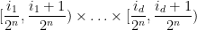
Exercise 14 (Metric entropy formulation of Jordan measurability) Define a dyadic cube to be a half-open box of the form
for some integers
. Let
denote the number of dyadic cubes of sidelength
that are contained in
be the number of dyadic cubes of sidelength
in which case one has


Exercise 15 (Uniqueness of Jordan measure) Let
be a map from the collection
of Jordan-measurable subsets of
Exercise 16 Let
Exercise 17 Let
be two polytopes in
can be partitioned into finitely many sub-polytopes which, after being rotated and translated, form a cover of
, with any two of the sub-polytopes in
(this is the Bolyai-Gerwien theorem), but false in higher dimensions (this was Dehn’s negative answer to Hilbert’s third problem).
The above exercises give a fairly large class of Jordan measurable sets. However, not every subset of
Exercise 18 Let
- Show that
of
- Show that
of
- Show that
of
- Show that the bullet-riddled square
, and set of bullets
, both have inner Jordan measure zero and outer Jordan measure one. In particular, both sets are not Jordan measurable.
Informally, any set with a lot of “holes”, or a very “fractal” boundary, is unlikely to be Jordan measurable. In order to measure such sets we will need to develop Lebesgue measure, which is done in the next set of notes.
Exercise 19 (Carathéodory type property) Let
be an elementary set. Show that
.
— 3. Connection with the Riemann integral —
To conclude these notes we briefly discuss the relationship between Jordan measure and the Riemann integral (or the equivalent Darboux integral). For simplicity we will only discuss the classical one-dimensional Riemann integral on an interval ![{[a,b]}](https://s0.wp.com/latex.php?latex=%7B%5Ba%2Cb%5D%7D&bg=ffffff&fg=000000&s=0&c=20201002)
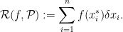
Definition 4 (Riemann integrability) Let
be a function. A tagged partition
of
, together with additional numbers
for each
. We abbreviate
as
. The quantity
will be called the norm of the tagged partition. The Riemann sum
of
with respect to the tagged partition
is defined as
We say that
and referred to as the Riemann integral of
by which we mean that for every
such that
for every tagged partition
.
If

Note that unbounded functions cannot be Riemann integrable (why?).
The above definition, while geometrically natural, can be awkward to use in practice. A more convenient formulation of the Riemann integral can be formulated using some additional machinery.
Exercise 20 (Piecewise constant functions) Let
, such that
on each of the intervals
. If
is independent of the choice of partition used to demonstrate the piecewise constant nature of
, and refer to it as the piecewise constant integral of

Exercise 21 (Basic properties of the piecewise constant integral) Let
be piecewise constant functions. Establish the following statements:
- (Linearity) For any real number
,
and
are piecewise constant, with
and
.
- (Monotonicity) If
pointwise (i.e.
for all
) then
.
- (Indicator) If
(defined by setting
when
and
otherwise) is piecewise constant, and
.
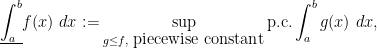
Definition 5 (Darboux integral) Let
of
where
ranges over all piecewise constant functions that are pointwise bounded above by
of
Clearly
. If these two quantities are equal, we say that

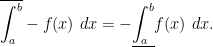
Note that the upper and lower Darboux integrals are related by the reflection identity
Exercise 22 Let
Exercise 23 Show that any continuous function
Now we connect the Riemann integral to Jordan measure in two ways. First, we connect the Riemann integral to one-dimensional Jordan measure:
Exercise 24 (Basic properties of the Riemann integral) Let
- (Linearity) For any real number
and
.
- (Monotonicity) If
.
- (Indicator) If
.
Finally, show that these properties uniquely define the Riemann integral, in the sense that the functional
is the only map from the space of Riemann integrable functions on
Next, we connect the integral to two-dimensional Jordan measure:
Exercise 25 (Area interpretation of the Riemann integral) Let
and
are both Jordan measurable in
where
denotes two-dimensional Jordan measure. (Hint: First establish this in the case when

Exercise 26 Extend the definition of the Riemann and Darboux integrals to higher dimensions, in such a way that analogues of all the previous results hold.

83 comments
Comments feed for this article
3 February, 2022 at 9:13 pm
sin
Dear Professor Tao:
For (2) of exercise 8, can one simply match the definition of upper and lower Riemman integeral with those of jordan outer and inner measure respectively and conclude that the measure does coincide with the area ?
[Yes, this will work – T.]
9 February, 2022 at 9:07 pm
sin
Dear professor Tao:
For (3) of exercise 11, I’m struggling to show that if L is a shear, then the measure of the image of the unit box is 1. Since L does not map boxes to boxes as the other two types of elementary transformations do, how should one proceeds from here ?
[Upper and lower bound the sheared box by a union of finitely many boxes. You can draw some pictures in two dimensions first to get intuition. -T]
23 February, 2022 at 3:59 pm
sin
Dear professor Tao:
I greatly appreciate all the patient responses from you. In Definition 7.4,1 of your analysis 2, the splitting property is used to test Lebesgue measurability, I wonder if the Carathéodory type property can be used to test Jordan measurability in a similar fashion?
17 June, 2022 at 2:49 pm
Anonymous
Dr. Tao: be a closed box in
  ,
, be a continuous function,
Let
and
consider the set
Someone mentioned that . i.e.
  is just the graph of
  ? If that’s the case, then Exercise 7(2) follows easily from (1). But the boundary should also include the bottom box
  , and the side surface set
 . The graph only covers the top of the set
  . Is this correct?
[Yes, but it is easy to manage the contribution of these additional regions for the purposes of establishing Exercise 7(2). -T]
4 March, 2024 at 4:38 pm
Anonymous
Dear professor Tao: Can you provide a bit hint on Exercise 9 (Jordan measurability of compact convex polytype)?
17 March, 2024 at 6:01 pm
Terence Tao
Try the case of a triangle in a plane first (perhaps assuming some of the sides parallel to the axes as an easier case), and then use the various Boolean algebra properties of Jordan measurability to handle other polygons. Then think about how to extend this argument to higher dimensions.